Mathematics
An Elbow or Nothing
elbow-helper detects the elbows of diminishing-returns curves, with quantified uncertainty. When the evidence is missing, it abstains.
 Try elbow-helper in the browser ↗
Start with an example anyone can picture. An online shop wants to sort its customers into groups that resemble each other: the bargain hunters, the Sunday regulars, the big-basket buyers. An algorithm can do that sorting, provided you tell it in advance how many groups to form. Two groups? The sorting stays coarse. Ten? Each group becomes so small it no longer means anything. Somewhere in between hides the right number.
To find it, you draw a curve. On the horizontal axis, the number of groups tried; on the vertical axis, a measure of the disorder left inside the groups. The curve drops fast at first, each added group soaks up a lot of disorder, then it flattens out: extra groups barely help anymore. The same diminishing-returns silhouette shows up when you ask when a model should stop training or at what budget an advertising channel saturates. The point where the curve stops paying off has an anatomical name: the elbow or knee1. Before it, every extra unit earns its keep; past it, you are just insisting.
Finding that point looks easy. Therein lies the trap: an elbow-detection algorithm always answers something, even on a perfect straight line or on pure noise. elbow-helper asks a harder question: is this candidate strong, unique, persistent, reproducible and unlikely under a no-elbow model? If a single one of those conditions fails, it abstains and says why. The whole pipeline runs at deraison.ai/elbow-helper, inside your browser: paste a curve and you will have the answer and its evidence before you finish reading this article.
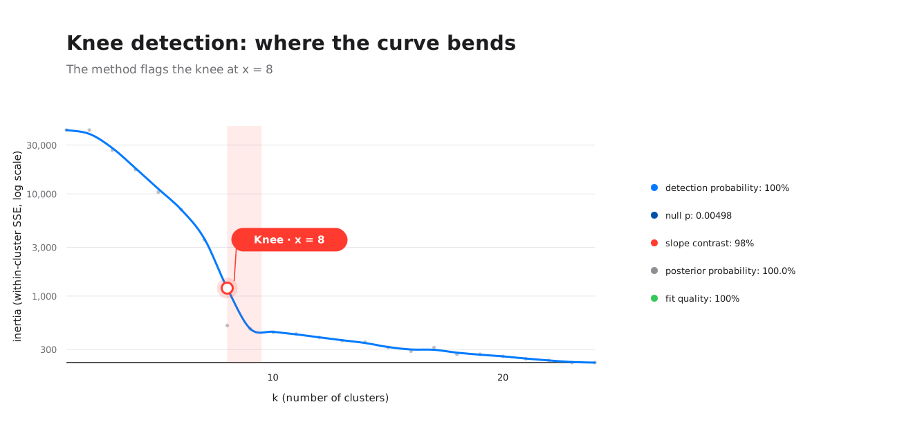
The textbook case: the inertia of a k-means, plotted against the number of clusters. k-means sorts points into a number of clusters fixed in advance; its inertia is the sum of the distances from each point to the center of its cluster. The detected elbow, its bootstrap interval and the quantified evidence beside it.
Motivation
Existing heuristics, starting with the Kneedle algorithm, the reference of the field,2, are excellent at proposing a location. They carry no notion of confidence, though: a point, with no error bar, no probability, let alone a right to withdraw. On a noisy curve, that lone point is easy to over-trust: you pick four clusters, size a cache, stop an experiment, on the strength of a noise artifact.
A radiologist looking at a blurry scan will hardly diagnose; they write that the image does not support a conclusion and order a second scan. A statistical procedure facing a noisy curve deserves the same restraint: conclude only what the data supports. The parallel has a limit: the radiologist exercises judgment, while the procedure applies thresholds calibrated once and for all, which makes it more predictable and less subtle at the same time.
elbow-helper's design priority is therefore
explicit: minimize false elbows, even at the price of abstaining more often. The output contract forces the
calling code to face this: either a ClearKnee with a position, a 90%
bootstrap interval (a bracket that aims to contain the true position in roughly nine cases out of
ten, without a coverage study having established it beyond the synthetic test bench) and
quantified evidence or a NoClearKnee with a
machine-readable reason code. No silent fallback to a doubtful estimate, much less a quiet guess:
abstention is handled, never
bypassed.
The tools that already exist split into three
camps. The knee locators, kneed3, kneebow4, Yellowbrick's visualizer5,
always answer with a point and can
never say "there is nothing here". The changepoint libraries, ruptures6
foremost, are excellent but handle a different question: how many breaks in a signal, with no notion of
diminishing returns. The third camp delegates the judgment to a human, by eye or through a language
model, which is not reproducible. elbow-helper's closest relative turns out not to be another knee
locator but R's segmented package7, which shares the same instinct: a
knee claim should come with an uncertainty, not just a coordinate. Explicit abstention, though, stays
rare across all of them: that is the main contribution. That comparison
comes with numbers: the ratings table and the map that summarizes its eleven criteria are at the end of
this article.
As for the scope, it is checkable rather
than proclaimed. The package is published on PyPI, the public index pip
install pulls Python libraries from, across eight successive releases from v0.1.0 to v0.1.7.
Every push is blocked until the 85 automated tests pass on Python 3.12 and the style checker returns a
clean verdict; a weekly sweep replays the same suite across the four supported Python versions, 3.10
through 3.13. Those 85 tests execute 96% of the package's lines.
The same pipeline is reachable through four doors: the Python library, a command line, a web interface other programs can put their questions to (an HTTP API), and a server exposing the same operations to a conversational assistant, through the tool-calling protocol known as the Model Context Protocol or MCP. All four are thin adapters over one shared core, so none of them can drift from what the library returns. Add to that the web app running the whole chain in the browser and a LaTeX note deriving every formula in the package, worked example included: ELBOW.pdf, with LIKELIHOOD.pdf covering the likelihood groundwork revisited below. The companion documents exist in English and in French, both kept in step with the code.
How it works
Before anything is searched for, the curve is put in order: non-finite points dropped, x values sorted and deduplicated, scales brought back to the unit square. That rescaling takes one precaution. Rather than anchoring its bounds on the lowest and highest points, it anchors them on the 5th and 95th percentiles: the values below which 5% and then 95% of the points fall. One outlier alone therefore cannot squash the rest of the curve against an edge.
A first shape screen follows. Is the curve monotone, that is, does it rise or fall without ever changing direction? A Spearman correlation8 answers that question by looking only at the ordering of the values, never at their magnitude; a magnitude-weighted monotonicity check doubles it. A curve with no clear trend is turned away at the outset, before any elbow is looked for.
The orientation of the curve need scarcely be declared. Direction is read off the sign of the trend. Convexity is read by comparing the curve to the chord joining its first and last point: above the chord it is concave, domed; below it is convex, hollowed like a bowl. All four combinations, concave or convex crossed with increasing or decreasing, are covered without the caller having to name the shape. A shape passed explicitly always overrides the inferred one.
The curve is clean and its orientation known; what is being looked for still has to be stated, starting with the word "elbow", which deserves an honest definition. Take a curve shaped like \(\sqrt{x}\), rising fast then settling down and subtract the diagonal joining its two endpoints: what remains is a bump, zero at both ends, largest where the curve pulls hardest away from a straight line. That peak is the elbow. After normalizing the data to the unit square, the difference curve reads:
Its local maxima, the points higher than their immediate neighbors, are the candidates. A sensitivity threshold then decides whether a peak is a real elbow or a mere wiggle: the candidate must dominate its neighborhood by a margin proportional to a parameter \(S\):
where the bar denotes the mean spacing between consecutive x values. The larger \(S\), the wider the required margin. This search is replayed over a whole grid of smoothing windows and sensitivities; only candidates that come back at the same place across scales survive: a real elbow holds up when the curve is blurred a little, a noise accident vanishes.
That peak search has a name and authors: it
is Kneedle2, described by Satopää,
Albrecht, Irwin and Raghavan in 2011, reimplemented here from scratch
in NumPy. Its traversal logic, orientation table and sensitivity threshold follow closely the
implementation choices of Kevin Arvai's kneed library3, released under
the three-clause BSD license and credited as such in the repository; elbow-helper carries no runtime
dependency on it. What this package adds lies elsewhere: in what a candidate is required to
survive before it gets named.
Model confirmation comes next. First requirement: the slope has to change and change in a way three stray points could not manufacture. That is what a Theil-Sen estimator9 measures. The least-squares method looks for the line that makes the sum of squared gaps as small as possible, so one wild value weighs very heavily on it. Theil-Sen goes another way. It computes the slope of every pair of points, then takes the median of those slopes, the middle value once they are ranked. A few wild points no longer decide the verdict.
That leaves the model itself to write. A real elbow is a change of slope: a straight line, then a different slope past the point \(k\). The hinge function \(\max(0, x - k)\), exactly zero before \(k\) and linear after, builds that broken line in one piece, with no jump:
The coefficient \(c\) carries the whole story of the bend: \(c = 0\) gives back a plain line with no elbow at all. The further \(c\) sits from zero, the sharper the slope breaks at \(k\). This broken model must then beat the plain line on two counts. First under blocked cross-validation10. The exercise is to hide part of the data, then see whether the model guesses what was hidden. Here whole contiguous chunks of the curve are held out, never isolated points: a single point is far too easy to guess from its immediate neighbors. Second on a score that compares the two models while accounting for their complexity; that score requires saying first what "fits better" means.
What "fits better" means: likelihood
A model fits the data well when, under that model, the observed data is unsurprising. That is the idea of likelihood. To make it computable, we commit to a model of the randomness. Each observed point departs from the theoretical curve by Gaussian noise, the bell-curve randomness that many small errors produce when they add up. Each departure is drawn independently of the others, with a typical spread written \(\sigma\), whose square \(\sigma^2\) is the variance. Every observation then receives a probability density, the number saying how expected that value was, larger the closer the point falls to the proposed curve.
The textbook definition multiplies those densities over the \(n\) points. That product raises a practical problem: multiplying \(n\) numbers smaller than one yields a quantity that collapses exponentially with \(n\), so a curve of 80 points and a curve of 800 stop being comparable. elbow-helper therefore takes the likelihood per observation: the geometric mean of the \(n\) densities. That mean is computed by multiplying the \(n\) numbers, then taking the \(n\)-th root of the result. The number of points stops weighing on this quantity:
Under the Gaussian model everything collapses in one stroke: a product of exponentials is the exponential of a sum; that sum divided by \(n\) is a mean. What remains is the mean squared error \(\mathrm{MSE}(\theta)\), the average of the squared gaps between observed points and fitted curve:
Taking the logarithm introduces no base here: it undoes the one the Gaussian density already carried.
That line holds a small revelation. At fixed variance, minimizing the mean squared error is exactly maximizing \(\ell\): ordinary least squares, learned as a geometric recipe and maximum likelihood, learned as a statistical principle, are one procedure rather than two. Replacing \(\sigma^2\) by the value the data best supports, \(\hat\sigma^2 = \mathrm{MSE}\), then exponentiating \(-2\ell\), lands on a quantity information theory calls perplexity. The word comes from language models, where perplexity reads as the number of words the model hesitates between at each step. Here, on numbers rather than words, it measures the same thing: the spread of values the model finds plausible. The lower it is, the less it hesitates:
Scaled back up to the whole sample, it gives the negative log-likelihood \(\mathrm{NLL}\), written through the residual sum of squares \(\mathrm{RSS}\), the mean squared error before dividing by \(n\):
Every BIC-family score (Bayesian Information Criterion)11 opens with that term and adds a penalty proportional to the number of parameters spent. The elbow costs parameters; it has to pay them back in fit.
One thing remains: making the quality of fit readable for a human. Comparing two models on fit alone would be rigged from the start: a model with more dials always clings closer to the data, right up to hugging the noise itself. The dials therefore have to be paid for. The reflex would be \(R^2\), the textbook fit score, which compares the model's error to the mean \(\bar y\)'s. Bad reference: \(\bar y\) is the constant that minimizes the error, the best trivial predictor there is, which is why an \(R^2\) can go negative. elbow-helper compares against a deliberately poor opponent instead, the observed point from which it is hardest to predict all the others:
The score is 1 for a perfect fit and 0 for a fit as bad as that worst constant. Since this reference is always worse than the mean, the bar to fall into negative territory sits far higher than \(R^2\)'s. That is the number printed in the diagnostic figure's legend. Three others sit beside it: the detection probability; the \(p\)-value, that is, the probability that chance alone would do as well, defined in the next section; and a model weight derived from the BIC. This last one is the odds between the two models, which the BIC gap yields through Kass and Raftery's approximation12. The wording matters: those odds hold under asymptotic assumptions, that is, ones valid in the limit of a large number of observations. Reading them as a posterior probability would further require priors over the two models, which nothing in the data supplies. So it is taken for what it is, a comparative weight.
The robustness trials
A model can win that duel on the observed data and still be a whim of the noise. Two trials guard against it. The bootstrap13: the entire search is replayed on copies of the curve obtained by reshuffling the residual noise. The name comes from the English expression about pulling yourself up by your own bootstraps: lacking other datasets, you make some out of the one you have. You subtract the fitted model from the curve, which leaves the gaps; you shuffle those gaps at random, then paste them back onto the model. Each copy is a curve you might have observed had chance drawn differently. To pass, the elbow must come back in at least 90% of the replays, at the same place, with a tight interval. And the null test: thousands of pure straight lines carrying the same noise level are simulated, measuring the probability \(p\) that a line with no elbow at all would produce, by chance, evidence as strong as the one observed.
That number deserves a pause, because it is the most misread quantity in all of statistics. The \(p\)-value does not give the probability that there is no elbow. It says the opposite: supposing there is none, how often chance alone would manufacture evidence as convincing as what we have in front of us. A \(p\)-value of 0.01 means a pure straight line would manage it once in a hundred tries. That is little, so the elbow is kept; it is not zero, so we can be wrong once in a hundred. That detour through simulation is not a luxury: under the no-elbow hypothesis the location \(k\) simply does not exist, so the classical tests lose the reference distribution they normally lean on14. Both bars must clear:
Only a candidate that clears every gate
becomes a ClearKnee. The diagnostic figure lays that case file out next
to the curve; on abstention, it switches to an honest state, curve grayed out and reason displayed,
never a marker implying more certainty than the data contains.
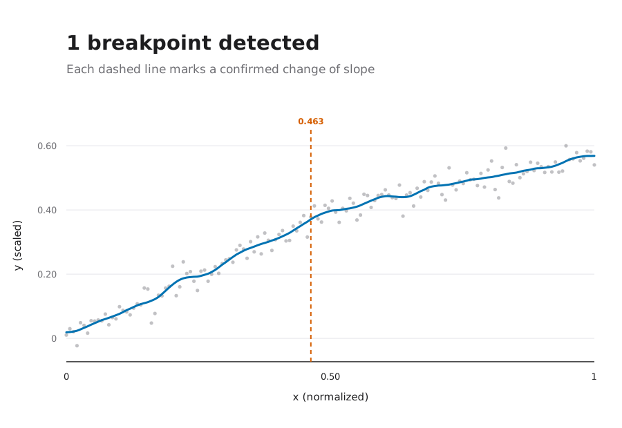
Low noise. The slope change is confirmed and placed at x = 0.463, marked by the dashed line. The true break sits at 0.5: the gap is the discretization onto the supplied points.
The next figure shows the same curve, the same break underneath, with stronger noise and nothing else changed.
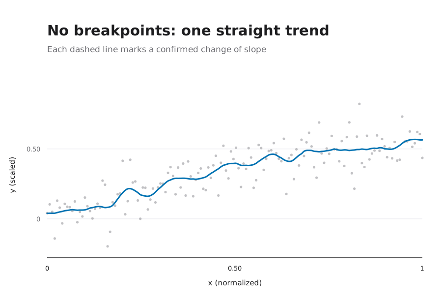
High noise, identical true shape. No break confirmed, so no marker drawn: the abstention reads off the figure itself.
What abstaining means
An abstention is not a silent failure: it is a return value, with a name. The function always returns one of two types, never anything else; the calling code has to look at which one before going on. Here are both answers as they print, on the same curve at two noise levels:
>>> from elbow_helper import robust_knee

>>> robust_knee(x, y)            # noise of standard deviation 0.02
ClearKnee(knee_x=0.3038, ci90=(0.3038, 0.3418), detection_rate=0.98, null_p=0.00498)

>>> robust_knee(x, y_noisy)      # same elbow, ten times the noise
NoClearKnee(reason='INCOMPATIBLE_GLOBAL_SHAPE')
The first line reads without documentation: elbow at 0.304, 90% bootstrap interval running from 0.304 to 0.342, elbow redetected in 98% of the replays, probability that an elbow-free straight line would do as well: five in a thousand. The second gives no position at all; that is deliberate: at that noise level the curve no longer even passes the shape screen, its trend being too faint to qualify.
Every refusal carries a stable code, readable by a machine as much as by a human. Those codes form a vocabulary settled in advance, fifteen reasons and not one more, on which a dashboard can count its abstentions and learn whether its curves are too short, too noisy or simply ambiguous.
| Returned code | What it says |
|---|---|
| Data preparation | |
| INVALID_INPUT | the inputs are unusable: mismatched lengths, no finite value, an unknown shape requested. |
| INSUFFICIENT_DATA | fewer points than the required minimum, twenty by default: too short for the later trials to mean anything. |
| ZERO_RANGE | the x axis does not vary: every point sits at the same place. |
| INCOMPATIBLE_GLOBAL_SHAPE | the curve does not have the shape announced or has no trend clear enough to infer one. |
| Candidate search | |
| NO_KNEE_CANDIDATES | the difference curve has no peak at all, at any smoothing scale. |
| ALL_CANDIDATES_WEAK | peaks exist, but none stands out enough against the local noise. |
| BOUNDARY_KNEE | the best candidate hugs one end of the curve, where an elbow cannot be told apart from an edge effect. |
| NO_PERSISTENT_CLUSTER | no candidate comes back to the same place when the smoothing scale changes. |
| MULTIPLE_PLAUSIBLE_KNEES | two elbows are equally defensible; answering would amount to a coin flip. |
| Statistical confirmation | |
| WEAK_SLOPE_CHANGE | the slope, once measured robustly, changes too little to deserve the word elbow. |
| SEGMENTED_MODEL_NOT_BETTER | the broken line fails to beat the plain line, on blocked cross-validation or on the BIC. |
| BOOTSTRAP_UNSTABLE | the elbow is recovered in only a minority of the reshuffled-noise replays. |
| BOOTSTRAP_MULTIMODAL | it is recovered often, but at two distinct places depending on the replay. |
| NULL_NOT_REJECTED | a straight line with no elbow, carrying the same noise, would too easily produce evidence this strong. |
| INTERNAL_NUMERICAL_FAILURE | a computation failed; the package says so instead of returning a doubtful number. |
The fifteen ways of saying no, in the order the pipeline can meet them.
That granularity has a practical
consequence: a refusal is actionable. INSUFFICIENT_DATA asks for a
longer grid; BOOTSTRAP_MULTIMODAL hints that there may be two elbows
rather than none and points at the plural search described below; NULL_NOT_REJECTED says the curve is pretty but that noise alone would
account for it.
Five doors, one verdict
A detector is only useful if it can be called
from wherever you work. elbow-helper therefore exposes the same pipeline through five surfaces. The
Python library for a notebook; the command line for a script or a continuous-integration chain (the
automatic checks replayed at every
code change); the
HTTP API for a service written in some other language than Python; the MCP server for a conversational
assistant;
the web app for anyone who would rather install nothing at all. The first four share one core and
expose the same four operations: knee (an elbow with its
uncertainty), elbow (the convex-decreasing k-means shortcut), diagnostics (the diagnostic figure, rendered as SVG, a vector drawing
format that stays sharp at any size) and locator (the bare locator,
with no case file). What one returns, the others return too, format aside.
Installing means choosing your door. The core depends on NumPy alone; the network surfaces are optional extras, in brackets, installed only if you use them:
$ pip install elbow-helper            # library + command line
$ pip install "elbow-helper[api]"     # + the HTTP API
$ pip install "elbow-helper[mcp]"     # + the MCP server (which pulls the API in)
The library
Two functions are enough. robust_knee takes a curve and infers its shape; robust_elbow is the shortcut for the k-means case, where the shape is
known in advance, convex and decreasing. The x values are optional: passing the y values alone amounts
to numbering them from zero to n minus one.
from elbow_helper import robust_knee, robust_elbow, RobustKneeConfig

res = robust_knee(x, y)                     # shape and direction inferred
res = robust_elbow(k_values, inertia)       # the k-means case, shape fixed
res = robust_knee(y)                        # implicit x: 0, 1, 2, ...

# More replays: slower, safer.
res = robust_knee(x, y, config=RobustKneeConfig(bootstrap_replicates=500,
                                                null_replicates=1000,
                                                random_seed=0))

if res.is_clear:
    print(res.knee_x, res.ci90, res.detection_rate, res.null_p_value)
else:
    print("no clear elbow:", res.reason)
Every threshold lives in RobustKneeConfig, a frozen structure: you do not edit a field, you make
a copy with config.with_(...). The shipped settings aim at the second
rather than at the decimal, a hundred bootstrap replays and two hundred draws under the null model; the
values above are validation-grade, five to ten times slower.
The command line
It follows the same four operations and answers in JSON, a structured text format programs read back without ambiguity, which pipes it straight into the usual tools. Data comes in as comma-separated values, as a NumPy file or as a CSV column named by its index:
$ elbow-helper knee --y-values 0,0.1,0.3,0.6,0.85,0.9,0.92,0.93,0.94,0.95
{
  "reason": "INSUFFICIENT_DATA",
  "diagnostics": {
    "curve": "auto",
    "direction": "auto",
    "n": 10,
    "min_samples": 20
  },
  "is_clear": false
}

$ elbow-helper elbow --x-npy k.npy --y-npy inertia.npy
$ elbow-helper knee --y-csv measures.csv:2 --config-json '{"bootstrap_replicates": 500}'
$ elbow-helper diagnostics --x-npy k.npy --y-npy inertia.npy > diagnostics.svg
The first command is worth a pause. The curve it receives has the right silhouette; any classic detector would have returned a number. Ten points are not enough to support an elbow claim: the answer is a documented refusal, stating how many points were supplied and how many would be needed, rather than an obliging estimate. The output contract crosses the doors intact.
The HTTP API
A server starts in one line and listens on
four routes named after the operations. The curve travels as JSON and so do the settings, inside a
config_overrides object; the diagnostics route returns the SVG itself, not a JSON wrapper around
it.
# uvicorn: the server that runs the Python application.
$ uvicorn elbow_helper.api:app --port 8000

$ curl -s -X POST localhost:8000/knee -H 'Content-Type: application/json' \
       -d '{"x": [0, 0.0127, ...], "y": [0.0043, 0.0361, ...],
            "config_overrides": {"random_seed": 0}}'
{"reason": "CLEAR_KNEE", "knee_x": 0.3038, "ci90": [0.3038, 0.3418],
 "detection_rate": 0.98, "null_p_value": 0.00498, "is_clear": true,
 "diagnostics": {...}}                       # response abridged
The MCP server
The MCP server is that same HTTP application,
with the four operations declared as tools a conversational assistant can discover and call, served at
/mcp:
$ uvicorn elbow_helper.mcp_server:app --port 8021
# The assistant connects to http://127.0.0.1:8021/mcp and finds
# four tools there: knee, elbow, diagnostics, locator.
The point goes beyond convenience. An assistant shown a curve will happily produce a plausible elbow, with nothing to contradict it. Wired to this tool, it gets a computed verdict, with an interval and a \(p\) value or a named refusal it cannot paraphrase into certainty.
The web app
The last surface asks for nothing: deraison.ai/elbow-helper runs the whole pipeline in the browser, on your data, without uploading it anywhere. Paste a curve and you get the same verdict and the same diagnostic figure as through the other four doors, in English or in French.
Several elbows: the dynamic program
A curve sometimes changes regime several
times, three pricing tiers on a demand curve say. The question then becomes: how many breaks and where?
That is what robust_knees, in the plural, answers; the change of
question forces a change of model. The curve is cut into pieces and each piece gets its own straight
line, fitted independently, with a visible jump allowed at the joint. This is a deliberate retreat from
the continuous hinge above: as soon as several breaks are free to move, a continuous fit no longer
decomposes into independent per-piece costs, since moving one break changes the condition its neighbors
must satisfy. And that decomposition is exactly what makes the search efficient enough to run on a
laptop.
First ingredient: the cost of one piece, computable in a single step. Fitting a line through \(m\) points and measuring its error looks like it requires walking over every point. It does not: six running totals suffice,
from which the least-squares slope and intercept follow and then the piece's error:
That last equality falls out of the least-squares normal equations; it says the cost of any stretch of the curve can be read off the totals without ever touching the points again. Computing those totals once costs \(O(n)\), time proportional to the number of points; every later segment cost then costs \(O(1)\), constant time, however long the curve is.
Second ingredient: the search itself. Trying every way to place \(k\) breaks among \(n\) points is out of reach: the number of ways to choose \(k\) spots among \(n\) runs into the billions as soon as the curve gets long. Dynamic programming sidesteps it by building the answer from sub-answers already known. Write \(C[k][t]\) for the minimal total cost of explaining the first \(t\) points with \(k+1\) segments:
The formula reads: for every possible position \(s\) of the last cut, add the best way of explaining the first \(s\) points with one break fewer, already computed and simply looked up, plus the cost of the final segment from \(s\) to \(t\); keep the minimum.
Why is looking up a sub-answer legitimate rather than recomputing everything? By contradiction, in one sentence. Suppose the best partition of the first \(t\) points has its last cut at \(s^\ast\), but its beginning, the first \(s^\ast\) points, is not the cheapest possible partition of that beginning. Then substituting the cheaper arrangement and keeping the last segment untouched yields a valid partition strictly cheaper than the best one. Contradiction. The start of an optimal solution is therefore optimal for its own sub-problem, which is Bellman's principle of optimality15.
Filling every cell costs \(O(k_{\max} \cdot n^2)\) operations, a manageable number where brute enumeration demanded an astronomical one; one stored arrow per cell lets the algorithm walk back through the table to recover the cut positions. This is the classic changepoint recursion. PELT16 is built on it too and speeds it up by pruning partitions that have become hopeless along the way. Here it is checked against exhaustive enumeration on small inputs rather than taken on faith.
Third ingredient: choosing the number of breaks. The more you add, the better the fit, down to the absurdity of one segment per point. A modified BIC17 settles it, adding to the negative log-likelihood a penalty that charges each break and also watches the length \(\ell_j\) of every segment:
The minus sign in front of the sum deserves an anecdote, because it says how this project works. The literature writes that term as an addition. Tested as written, it produces the opposite of its intended effect: the term being always negative, adding it rewards uneven partitions instead of penalizing them. The subtractive form does penalize short and uneven segments, matching the stated intent. The convention kept here is therefore the one the tests confirm; the discrepancy is documented rather than hidden. What is not settled should be said too: a sign that looks flipped sometimes comes from a different definition of the likelihood, from a score minimized instead of maximized, or from a length normalized another way. Establishing the term-by-term correspondence with the original parameterization would take an appendix the repository has yet to write. So this is a measured disagreement, not a correction to the literature.
The winner is finally confirmed by a permutation test: thousands of reshuffles of the curve, none carrying any true break, must almost all do worse than the real fit. Since running more tests means more chances to get lucky, a Bonferroni correction tightens each test's bar in proportion to how many are run18.
One nuance separates the singular from the plural; it matters. In the plural, an empty answer is not an abstention but a conclusion: this curve has no real break, a verdict that cleared exactly the gates a non-empty answer would have had to clear. Only a preprocessing failure, invalid input, too little data, zero range, returns an error object instead of a list of breaks.
Those choices, the dynamic program over the greedy search, the subtractive sign, the permutation confirmation, were settled by measurement. Ten combinations were put in competition. On one hand, two ways of searching: the dynamic program, which examines every partition and the greedy approach, which lays its breaks down one at a time and never revisits them. On the other, five ways of choosing how many breaks there are, from the bare BIC to the permutation gate. Two times five. Each method handled three hundred synthetic curves: a hundred points each, twenty-five replicates for every combination of four true break counts, zero to three and three noise levels. The labels on the two figures below read as follows: DP for the dynamic program and Greedy for the greedy search; BIC for the bare criterion, mBIC_add and mBIC_sub for the two signs of the segment-length term, ICL for a neighbouring Bayesian criterion that also charges for the uncertainty of the partition19, FWER for the Bonferroni-corrected permutation gate.
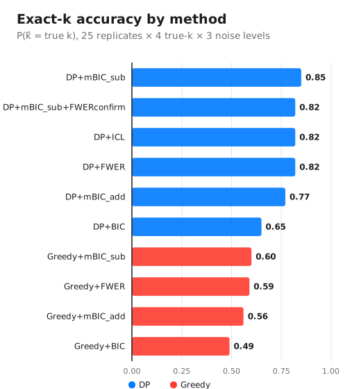
Probability of recovering the true number of breaks. The top five methods all rest on the dynamic program; the bottom five are their greedy twins.
Two lessons read straight off that ranking. The exhaustive search beats its greedy twin every time and by a wide margin: 0.85 against 0.60 for the same criterion. The mechanism is the one the binary-segmentation literature describes20: the greedy search commits early to an imperfect cut. Every cut that follows then goes into repairing that error rather than describing the curve. The sign of the segment-length term, the anecdote told above, comes with a number too: 0.85 for the subtractive form against 0.77 for the literature's additive one.
That leaves the sin this project cares about most: inventing a break where there is none. The second figure measures exactly that, on curves drawn deliberately flat.
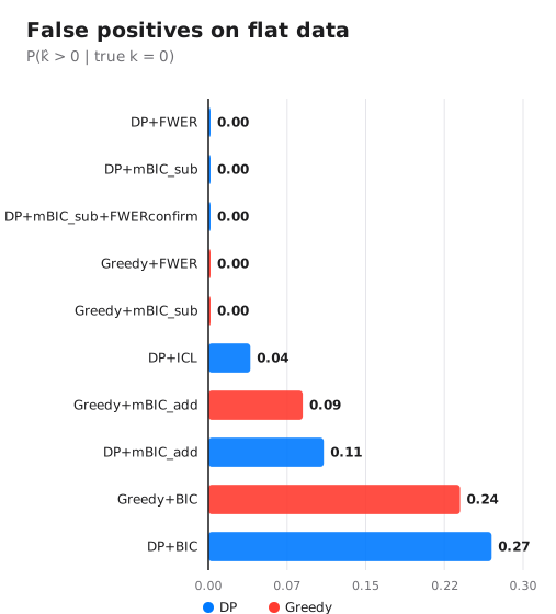
Probability of announcing at least one break on a curve that has none. The bare BIC is wrong one time in four, the drift theory has long ascribed to it21; the subtractive form and the permutation gate are never wrong across these three hundred curves.
The limit is shared by every method and deserves stating: at high noise with three true breaks, none of them recovers all three, the best hovering around 1.8 breaks announced on average. The error therefore runs toward fewer elbows, never toward more, which is exactly the direction this package accepts being wrong in. These numbers hold for that family of synthetic curves and for it alone; the full protocol is published in the repository, with the detailed table by noise level22.
The whole thing stands on a single computational dependency, NumPy: the locator is rewritten from scratch; the diagnostic figure is hand-authored SVG, with no plotting library. Every formula in the chain, from normalization to the permutation test, is derived step by step in the repository's mathematical note, ELBOW.pdf23, written intuition-first, with a worked example before every formula. The likelihood groundwork used above is treated separately, in LIKELIHOOD.pdf24, since it owes nothing to curve fitting.
What it does not do
A project that claims caution has to state its own limits or it commits the overconfidence it holds against the others.
The smoother assumes x values that are regularly spaced or nearly so: a curve sampled any which way would defeat it. The reported position is discretized onto the supplied points. At modest sample sizes the elbow can therefore land a few samples away from the truth. On the family of synthetic curves used as a test bench, the median error stays below about 5% of the x range. The straight-line null and the residual bootstrap make another assumption: noise that is roughly homoscedastic, that is, of constant variance from one end of the curve to the other and uncorrelated from one point to the next. The variants that drop that assumption remain to be written.
Finally, the thresholds are values calibrated on a documented family of curves, not universal constants: 90% redetections and a \(p\) value at 1% are defensible choices, not laws of nature. The package is at v0.1.x; its author says so: recalibrate on your own family of curves and noises if your decision depends on it. No method working on finite data is infallible; this one merely makes its assumptions checkable.
Conclusion
A detector that abstains serves you better than a detector that always answers. "No clear elbow" is real information: it keeps you from sizing a system, stopping an experiment or settling a budget on a fold of randomness. The displayed confidence is paid for in abstentions; that is a trade I stand by.
elbow-helper installs in one line, pip install elbow-helper and can be tried with nothing installed in the
online
sandbox, where the full pipeline runs in your browser without uploading your data. The code, the
examples, the comparison with neighbouring tools and the mathematical notes all live in the GitHub repository. Bring a curve; you will leave with a
defensible elbow or with a good reason not to believe in one.
The landscape, tool by tool
That leaves the map itself. The repository rates eight ways of looking for an elbow on eleven criteria; the rating is about the job this package does, reporting an elbow only when the evidence carries it: no tool is marked down for excelling at some other job.
| Elbow Detection Tool | Noise robustness | Shape inference | Explicit abstention | Multiple breakpoints | Significance test | Uncertainty | Model selection | Light dependencies | One-call ease | Reproducible | Published maths |
|---|---|---|---|---|---|---|---|---|---|---|---|
| elbow-helper | ⭐️⭐️⭐️⭐️⭐️ | ⭐️⭐️⭐️⭐️⭐️ | ⭐️⭐️⭐️⭐️⭐️ | ⭐️⭐️⭐️⭐️⭐️ | ⭐️⭐️⭐️⭐️⭐️ | ⭐️⭐️⭐️⭐️⭐️ | ⭐️⭐️⭐️⭐️⭐️ | ⭐️⭐️⭐️⭐️⭐️ | ⭐️⭐️⭐️⭐️⭐️ | ⭐️⭐️⭐️⭐️⭐️ | ⭐️⭐️⭐️⭐️⭐️ |
| kneed | ⭐️⭐️⭐️⭐️⭐️ | ⭐️⭐️⭐️⭐️⭐️ | ⭐️⭐️⭐️⭐️⭐️ | ⭐️⭐️⭐️⭐️⭐️ | ⭐️⭐️⭐️⭐️⭐️ | ⭐️⭐️⭐️⭐️⭐️ | ⭐️⭐️⭐️⭐️⭐️ | ⭐️⭐️⭐️⭐️⭐️ | ⭐️⭐️⭐️⭐️⭐️ | ⭐️⭐️⭐️⭐️⭐️ | ⭐️⭐️⭐️⭐️⭐️ |
| ruptures | ⭐️⭐️⭐️⭐️⭐️ | ⭐️⭐️⭐️⭐️⭐️ | ⭐️⭐️⭐️⭐️⭐️ | ⭐️⭐️⭐️⭐️⭐️ | ⭐️⭐️⭐️⭐️⭐️ | ⭐️⭐️⭐️⭐️⭐️ | ⭐️⭐️⭐️⭐️⭐️ | ⭐️⭐️⭐️⭐️⭐️ | ⭐️⭐️⭐️⭐️⭐️ | ⭐️⭐️⭐️⭐️⭐️ | ⭐️⭐️⭐️⭐️⭐️ |
| kneebow | ⭐️⭐️⭐️⭐️⭐️ | ⭐️⭐️⭐️⭐️⭐️ | ⭐️⭐️⭐️⭐️⭐️ | ⭐️⭐️⭐️⭐️⭐️ | ⭐️⭐️⭐️⭐️⭐️ | ⭐️⭐️⭐️⭐️⭐️ | ⭐️⭐️⭐️⭐️⭐️ | ⭐️⭐️⭐️⭐️⭐️ | ⭐️⭐️⭐️⭐️⭐️ | ⭐️⭐️⭐️⭐️⭐️ | ⭐️⭐️⭐️⭐️⭐️ |
| KElbowVisualizer | ⭐️⭐️⭐️⭐️⭐️ | ⭐️⭐️⭐️⭐️⭐️ | ⭐️⭐️⭐️⭐️⭐️ | ⭐️⭐️⭐️⭐️⭐️ | ⭐️⭐️⭐️⭐️⭐️ | ⭐️⭐️⭐️⭐️⭐️ | ⭐️⭐️⭐️⭐️⭐️ | ⭐️⭐️⭐️⭐️⭐️ | ⭐️⭐️⭐️⭐️⭐️ | ⭐️⭐️⭐️⭐️⭐️ | ⭐️⭐️⭐️⭐️⭐️ |
| R segmented package | ⭐️⭐️⭐️⭐️⭐️ | ⭐️⭐️⭐️⭐️⭐️ | ⭐️⭐️⭐️⭐️⭐️ | ⭐️⭐️⭐️⭐️⭐️ | ⭐️⭐️⭐️⭐️⭐️ | ⭐️⭐️⭐️⭐️⭐️ | ⭐️⭐️⭐️⭐️⭐️ | ⭐️⭐️⭐️⭐️⭐️ | ⭐️⭐️⭐️⭐️⭐️ | ⭐️⭐️⭐️⭐️⭐️ | ⭐️⭐️⭐️⭐️⭐️ |
| Manual eyeballing | ⭐️⭐️⭐️⭐️⭐️ | ⭐️⭐️⭐️⭐️⭐️ | ⭐️⭐️⭐️⭐️⭐️ | ⭐️⭐️⭐️⭐️⭐️ | ⭐️⭐️⭐️⭐️⭐️ | ⭐️⭐️⭐️⭐️⭐️ | ⭐️⭐️⭐️⭐️⭐️ | ⭐️⭐️⭐️⭐️⭐️ | ⭐️⭐️⭐️⭐️⭐️ | ⭐️⭐️⭐️⭐️⭐️ | ⭐️⭐️⭐️⭐️⭐️ |
| Ask an LLM | ⭐️⭐️⭐️⭐️⭐️ | ⭐️⭐️⭐️⭐️⭐️ | ⭐️⭐️⭐️⭐️⭐️ | ⭐️⭐️⭐️⭐️⭐️ | ⭐️⭐️⭐️⭐️⭐️ | ⭐️⭐️⭐️⭐️⭐️ | ⭐️⭐️⭐️⭐️⭐️ | ⭐️⭐️⭐️⭐️⭐️ | ⭐️⭐️⭐️⭐️⭐️ | ⭐️⭐️⭐️⭐️⭐️ | ⭐️⭐️⭐️⭐️⭐️ |
The repository's eleven criteria, from one to five stars. The highlighted row is the package this article is about.
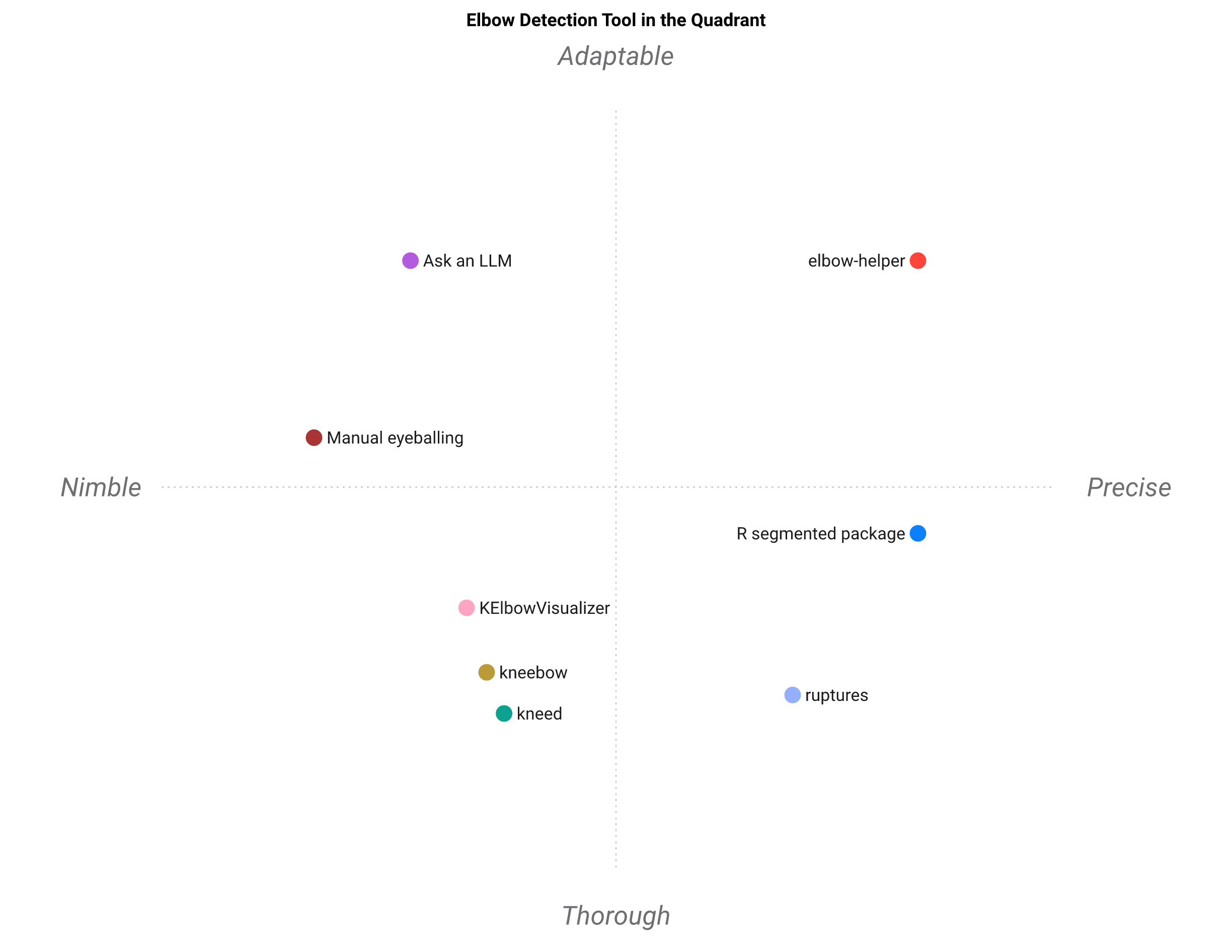
The same table seen from above: eleven columns summarized into two axes by principal component analysis, the technique that projects a table onto the two directions that best summarize it, the axes then named by hand. elbow-helper sits alone in the precise and adaptable corner. Map drawn by Standpoint, the tool that reads a ratings table and draws its map.
- elbow-helper: the only one here that can refuse to answer: persistence across smoothing scales, bootstrap, null-model test, then either an elbow with its interval or a named abstention code.
- kneed: the reference implementation of Kneedle, deterministic and immediate. A point, always, with no error bar and no way out.
- kneebow: the same geometric idea, obtained by rotating the curve. Very light on dependencies, but it commits on every call.
- KElbowVisualizer: the most common way to read a k-means elbow in practice: plot it, look at it. A visualization tool built for one curve shape, inheriting scikit-learn and matplotlib.
- ruptures: the right tool when the question really is “how many breakpoints and where”, with PELT and binary segmentation already in place. Diminishing returns mean nothing to it.
- R segmented package: statistically the most rigorous: broken-line regression, standard errors, Davies test, multiple breakpoints. It asks for R and real statistical fluency.
- Manual eyeballing: a careful eye can say “I see nothing clear here”, which most tools cannot. But the judgement reproduces neither across people nor at scale.
- Ask an LLM: describes a shape in words fluently and hedges when asked, with no calibrated uncertainty, no checkable derivation, let alone two identical answers.
Bibliography
Here are the works this package depends on, ordered as the article uses them. Each note says what the source establishes and where it does its work here; the classics are cited for the standard result they ground, the repository's own notes for the derivations and measurements they carry.
- Thorndike, R. L. (1953). "Who belongs in the family?", Psychometrika, 18(4), 267-276. 10.1007/BF02289263 A presidential address to the Psychometric Society, commonly given as the first statement of the elbow criterion: plot a measure of spread against the number of groups and look for the bend. It sets the question this article lives on, without offering a decision rule.
- Satopää, V., Albrecht, J., Irwin, D. and Raghavan, B. (2011). "Finding a Kneedle in a Haystack: Detecting Knee Points in System Behavior", ICDCSW, IEEE. Defines the knee as the maximum gap to the chord after normalization, with a sensitivity threshold: the locator rewritten here. Its limit is in its own statement: it proposes a location, it does not say whether the knee exists.
- Arvai, K. kneed, Python library, three-clause BSD license. github.com/arvkevi/kneed The reference Python implementation of Kneedle. Its traversal logic, orientation table and sensitivity threshold guided elbow-helper's NumPy rewrite, which carries no runtime dependency on it.
- kneebow, Python library, MIT license. github.com/georg-un/kneebow Rotates the curve and takes the extremum of the rotated data. Representative of the camp that always answers with a point and can never keep quiet.
- Bengfort, B. and Bilbro, R. (2019).
"Yellowbrick: Visualizing the Scikit-Learn Model Selection Process", Journal of Open Source Software, 4(35), 1075. 10.21105/joss.01075 A
visual-diagnostics library for scikit-learn, including the
KElbowVisualizerthat plots inertia and marks an elbow. The tool aims at reading by eye, not at a quantified decision. - Truong, C., Oudre, L. and Vayatis, N.
(2020). "Selective review of offline change point detection methods", Signal Processing, 167, 107299. arxiv.org/abs/1801.00718 A review that sorts changepoint detection into three parts,
a cost function, a search method and a constraint on the number of changes; it accompanies the
ruptureslibrary. That is the frame this article's multi-elbow part inherits, on a question adjacent to, but distinct from, diminishing returns. - Muggeo, V. M. R. (2003).
"Estimating regression models with unknown break-points", Statistics in
Medicine, 22(19), 3055-3071. 10.1002/sim.1545 Estimates a breakpoint's position by successive
linearizations and returns a standard error with it, hence an interval. It is elbow-helper's
closest relative on the idea that a knee claim should carry its uncertainty; the R package
segmentedis its implementation. - Spearman, C. (1904). "The Proof and Measurement of Association between Two Things", American Journal of Psychology, 15(1), 72-101. A correlation computed on ranks rather than on values. It serves here as a shape screen, indifferent to scale and little disturbed by a few extreme points.
- Theil, H. (1950). "A Rank-Invariant Method of Linear and Polynomial Regression Analysis", Proceedings of the Royal Netherlands Academy of Sciences, 53; Sen, P. K. (1968). "Estimates of the Regression Coefficient Based on Kendall's Tau", Journal of the American Statistical Association, 63(324), 1379-1389. Together they establish the slope estimator built from the median of all pairwise slopes. It is what lets the pipeline demand a slope change without letting a handful of outliers decide the verdict.
- Arlot, S. and Celisse, A. (2010). "A survey of cross-validation procedures for model selection", Statistics Surveys, 4, 40-79. 10.1214/09-SS054 A review that carefully separates what is proved from what is merely observed about cross-validation and shows that the shape of the held-out blocks has to match the dependence in the data. That is the justification for holding out contiguous stretches here.
- Schwarz, G. (1978). "Estimating the Dimension of a Model", The Annals of Statistics, 6(2), 461-464. Establishes the BIC: a penalty equal to the number of parameters times the logarithm of the number of observations, derived as an approximation to the marginal likelihood. It is the score the broken line has to beat to earn its elbow.
- Kass, R. E. and Raftery, A. E. (1995). "Bayes Factors", Journal of the American Statistical Association, 90(430), 773-795. Gives the approximation by which a BIC gap reads as odds between two models and the interpretation scale that goes with it. That is the posterior probability shown in the diagnostic figure's legend.
- Efron, B. (1979). "Bootstrap Methods: Another Look at the Jackknife", The Annals of Statistics, 7(1), 1-26. Introduces resampling as a stand-in for a sampling distribution nobody can write down. Here it is the residual noise that gets reshuffled, to measure how often and where the elbow comes back.
- Davies, R. B. (1977). "Hypothesis testing when a nuisance parameter is present only under the alternative", Biometrika, 64(2), 247-254. 10.1093/biomet/64.2.247 Treats exactly the elbow's difficulty: a parameter that exists only if the alternative hypothesis is true, here the location \(k\). The likelihood-ratio test loses its usual asymptotic distribution there, which is why the \(p\)-value is simulated rather than read off a table.
- Bellman, R. (1957). Dynamic Programming, Princeton University Press. The canonical source of the principle of optimality: the start of an optimal solution is optimal for its own sub-problem. That is what licenses the recursion used here to place several breaks.
- Killick, R., Fearnhead, P. and Eckley, I. A. (2012). "Optimal Detection of Changepoints With a Linear Computational Cost", Journal of the American Statistical Association, 107(500), 1590-1598. PELT: the same exact recursion, sped up by pruning that permanently discards partitions which have become hopeless, giving a linear cost under conditions on the penalty.
- Zhang, N. R. and Siegmund, D. O. (2007). "A Modified Bayes Information Criterion with Applications to the Analysis of Comparative Genomic Hybridization Data", Biometrics, 63(1), 22-32. Introduces the modified BIC whose extra term watches segment lengths. It is the reference whose sign, taken at face value first, had to be corrected here once its real effect was measured.
- Dunn, O. J. (1961). "Multiple Comparisons Among Means", Journal of the American Statistical Association, 56(293), 52-64. 10.1080/01621459.1961.10482090 Establishes and puts to work the inequality statistics calls Bonferroni: dividing the threshold by the number of tests bounds the risk of being wrong at least once. Used here as soon as several break counts are put to the test.
- Biernacki, C., Celeux, G. and Govaert, G. (2000). "Assessing a Mixture Model for Clustering with the Integrated Completed Likelihood", IEEE Transactions on Pattern Analysis and Machine Intelligence, 22(7), 719-725. The ICL criterion, which adds to the BIC a penalty on the uncertainty of the assignment. A competitor in the comparison, where it reaches 0.82 accuracy and a 4% false-positive rate.
- Fryzlewicz, P. (2014). "Wild Binary Segmentation for Multiple Change-Point Detection", The Annals of Statistics, 42(6), 2243-2281. Analyses the flaw in greedy searches, which commit to a cut too early and propagate the error and fixes it with randomly drawn intervals. This article's comparison recovers that flaw: every greedy method stays below its exhaustive twin.
- Yao, Y.-C. (1988). "Estimating the number of change-points via Schwarz' criterion", Statistics and Probability Letters, 6(3), 181-189. Studies the BIC applied to the number of changepoints and documents its tendency to keep too many. The 27% false-positive rate measured here is one instance of that, on piecewise-linear curves.
- Harchaoui, W. (2026). Multi-knee method comparison: results, research note in the elbow-helper repository. research/multiknee/RESULTS.md The full protocol behind the comparison above: ten methods, three hundred curves each, results broken down by break count and noise level, runtimes and the six conclusions drawn from them.
- Harchaoui, W. (2026). ELBOW: Noise-Robust Knee and Elbow Detection, technical note in the elbow-helper repository. doc/ELBOW-en.pdf Derives every formula in the package step by step, from normalization to the permutation test, intuition and a worked example before each one. It is the long version of everything this article compresses.
- Harchaoui, W. (2026). LIKELIHOOD, technical note in the elbow-helper repository. doc/LIKELIHOOD-en.pdf The likelihood groundwork revisited above: why the per-observation likelihood, the geometric mean of the densities, rather than the raw product and how the same construction reads on a classification model.
To close, three readings friendlier than a journal paper. My favourite AI books supply the annotated panorama the next two come from. The Elements of Statistical Learning by Hastie, Tibshirani and Friedman covers model selection and cross-validation at large. Information Theory, Inference and Learning Algorithms by MacKay traces the link, sketched here, between likelihood, coding and perplexity.