Artificial intelligence
The model does not write the number
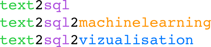
Four plain-language questions put to a company database: a number, a prediction, a forecast, a chart. Every time, the language model writes the query; the database is what answers.
You ask a language model a question about your data. A language model is the program that has learned to read and write text, the one behind chat assistants. It answers with a number. The number is plausible. It is wrong. Hardly anyone signs off on a board decision on the strength of a plausible number. That single fact blocks more enterprise deployments than budget and regulation combined.
Three words are enough to follow the whole article. A database is a set of large tables, cousins of spreadsheets: a table of customers, a table of invoices, thousands of rows each. A query is a question put to those tables in a language built for the job, the Structured Query Language, SQL: rigid, free of double meanings, saying exactly which rows to take and what to do with them. The language model understands plain language; it can also write SQL. Everything that follows sits in that meeting point.
So the answer to the wrong number is not to ask more politely. It is to take away the model's ability to be wrong about the number at all: it does not write the answer, it writes the query. The database answers what it holds, no more and no less. The distinction looks like nothing; it changes the nature of the error. A wrong query is visible, loggable, replayable, fixable. A hallucinated number is invisible, because it looks exactly like a correct one.
This article follows four questions really
put to an enterprise deployment, in the order they come up in a meeting: last month's number, a
row-by-row prediction, a three-month forecast, then a chart. Three storeys on one foundation, each named
like an address: txt2sql for the number, txt2sql2ml for the prediction, txt2sql2viz for the figure. The first storey is well-trodden industry
ground; the other two are far rarer. Those are the ones I built.

The foundation is the same at all three storeys: the question becomes a query, the query is parsed before it runs, the database answers. Only the last link changes.
"How many invoices are overdue?"
The answer lands in two seconds: thirteen. And, unfolded underneath it, the query that produced it.
SELECT COUNT(*) FROM invoices WHERE status = 'overdue' LIMIT 500
Even without ever having read SQL, you can
decipher it: count (COUNT) the rows of the invoices table (invoices) whose status equals overdue,
and never bring back more than five hundred of them (LIMIT 500).
Showing that query is not a flourish of transparency. It is the evidence: a reader who knows the database can read it, dispute it, replay it. The number is not there to be believed, it is there to be checked.
Writing SQL in general is something a recent
language model does very well. The difficulty lies wholly elsewhere: writing the right query for this database. The right table names, the right joins (the operation that
links two tables through a shared column, invoices to their customers for instance), above all the right
filter values. Is an unpaid invoice's status spelled overdue, unpaid or 3? A model that does not know
the schema, the map of the database, the
list of its tables and their columns, invents names that are plausible and wrong. That is where all the
value of a text-to-SQL tool sits: anchoring generation in the reality of one given database.
Two families of solution exist. Fine-tuning sends the model back to school: its training is resumed on the customer's data until it knows them by heart. Expensive, slow, to be redone at every schema change. Retrieval-augmented generation (RAG) leaves the model untouched: for each question, it slips the model a revision sheet, the few pieces of context that matter for that precise question2. Vanna, the open source reference on this ground, belongs to the second family1.
One point is disconcerting from the outset, the most important of all: in Vanna, the word "train" means filling a knowledge base that the system consults at answer time. Nothing changes inside the model itself: none of its internal dials, its weights, is touched. You file texts away in a kind of library, you retrieve the ones that talk about the same thing as the question asked, even phrased differently, you paste them into the prompt, the text handed to the model3.
Three materials, in the reverse order of intuition
Three kinds of content go into that library. Intuition gets their relative weight wrong.
The table
structure comes first in time. It is each table's CREATE TABLE,
its identity card in effect: its name, its columns, the type of each (number, text, date) and its
keys, those columns that link it to other tables. It teaches the model what exists and stops it
inventing.
One table per entry, so each is retrieved independently when a question touches it.
The business
glossary encodes what the structure does not say: the definition of a measure, in-house
vocabulary, the meaning of coded values. One self-contained statement per entry, phrased the way a user
would say it. "Revenue excluding tax on orders is the sum of orders.total_ht_eur." This is where the largest gains sit, precisely
where a model without context goes wrong most often.
The question-to-query pairs come last in the order of work and first in the order of payoff. A question in plain language, the correct query beside it. Vanna's documentation says it without hedging: their quality is the single largest determinant of the result1. The mechanism explains why. For each question, the system shows the model only the few closest cards; the rest of the library does not exist for it. One correct example close to the question asked is therefore worth a thousand distant ones. You curate for coverage, not for volume: twenty to a hundred verified pairs are enough to start, provided they are the right ones, provided they cover the families of query users will produce, from counting to joining, from filtering on a coded value to ranking the top N9. That order of magnitude holds for a schema of this size; it is not a general rule. It depends on the number of tables, on how ambiguous the business vocabulary is, on the number of functional domains, and above all on the real distribution of the questions asked.
Two curation rules (curation being the
careful
sorting of what enters the library) dominate. Always verified SQL, meaning
executed and confirmed correct: a wrong pair teaches the system to produce wrong SQL. And never
SELECT *, the query that brings back every column without naming any:
it teaches nobody a single column name.
Two locks between the model and the database
The model produces a query, nothing more. Execution happens elsewhere, under a read-only database role, an account allowed to consult the tables and never to change them, behind guardrails that parse the query before running it. Parsing here means breaking the query down the way you diagram a sentence in grammar class, subject, verb, complements: that breakdown is called a syntax tree4. Reading that tree is what lets the pipeline refuse anything that is not a plain read. The separation is a security decision, not an aesthetic one: the component that talks to the model never has the right to write to the database.
The second lock was born of a precise
failure, dated 4 September 2026. Until then the model received column names and types, never their
domain, the set of values they really hold. So it wrote WHERE status = 'confirmed' against the invoices table. Syntactically
valid. Accepted by the guardrails. Executed without error. Zero rows. The real values were paid, overdue and sent; confirmed belonged to the orders
table, a different table. The user saw an empty result, with scarcely a clue as to why.
That flaw is fixed from both ends. As prevention, the pipeline goes after low-cardinality columns, the ones that take only a handful of distinct values: a status, a category, never an amount. Each now carries its real domain, read from the database, then written into the context given to the model. First the enumerated types, the columns whose exact list of allowed values the database knows by construction; then the text columns the database statistics declare low-cardinality, whose domain is re-read with a bounded query. A column with no statistics is never probed: no domain beats a wrong domain.
As a cure, a query that runs without error but returns no rows, while filtering on a value spelled out in the query itself (a literal) that is absent from the known domain, no longer hands back a silent blank. A second attempt is made with the real values given to the model; failing that, the answer names the column, the invented literal and the real domain.
Proving that all this work is worth something
This is the step people skip. It is the only one that proves the curation paid. You hold back a few pairs you never file into the library: a control set. The principle is the one behind every exam: you do not grade a student on the exercises whose answer key they are holding. Measured on questions already filed away, accuracy says nothing beyond the system's ability to regurgitate a memorised example.
Three ways of scoring are available, from weakest to most reliable. Valid-SQL rate is a mere guardrail: a query can be valid and wrong. Exact textual match, which compares the two queries character by character, badly undercounts accuracy, since two correct queries are almost always written differently5. The right measure is execution match: you run both the generated query and the reference query read-only, then compare the results, order aside. It is the measure used by the field's benchmarks, the public question sets every team scores itself against, Spider6 and BIRD7, because it judges the answer delivered, which is the only thing that matters.

On the control set, the business glossary and the worked examples take the share of correct answers from 62.5 % to 87.5 %. Three examples added on the two lagging families, joins and one filter, take it to 100 %. Replayed on three database sizes, the same measurement gives the same result: it is the library of examples that moves the score, not the data volume. One caveat without which these figures get over-read: the control set is small; scores move across it in steps of 12.5 points, which says enough about how fine-grained it is. That 100 % means nothing is missing on those questions. It does not say the pipeline is correct in general; a case study is not a benchmark.
One global score, on its own, hides the family of queries that fails8. So you break the score down by family: counts, joins, filters, rankings. That reading drives what comes next: weak joins call for join examples, not for a bigger model. That is exactly what happened here; it is the jump from 87.5 % to 100 % on the chart.
"Which customers are at risk of leaving and how confident are you?"
An exact number answers a question about the past. How much did we invoice last month, which customers went over budget. It does not answer the one the executive asks next, the one that looks ahead and decides something. Until now that second question meant a project of several months handed to data specialists, per customer and per question.
The idea that changes this is simple. The query no longer brings back a number: it brings back a table whose last column is the question, known for some rows, empty for the ones to predict.
| Customer | Segment | Recency | Frequency | Tickets | Left? |
|---|---|---|---|---|---|
| Studio Moreau | SMB | 12 d | 8 | 1 | no |
| Fabrique Horizon | Enterprise | 190 d | 1 | 4 | yes |
| Maison Central | SMB | 45 d | 5 | 0 | ? |
One question, one query: the gaps fill in. SQL cannot predict; it can fetch the right shape of table.
That table holds both the example and the question. Which is exactly what a tabular foundation model knows how to read. Such a model was pre-trained once and for all, at its laboratory, on millions of synthetic tables, made up for the exercise. It does not know your data; it knows how tables behave, the way a grader who has marked thousands of papers spots a mistake at first glance on a paper they have never seen. Show it this one, and it fills the gaps in a single pass: no training on your data, no internal dial adjusted, no model to store, let alone a GPU to rent.
This is called in-context learning. The analogy that lands is one everybody has already lived: giving a chat assistant an example inside the conversation itself and watching it catch on without retraining10. The analogy has an instructive limit: text reads left to right, a table has no order, neither across rows nor across columns. That is the very problem these models had to solve.
The direct consequence: zero training projects, zero artefacts to maintain. The day you plug in a new customer, there is no model to retrain. One and the same code covers classification (predicting a category: will leave, will stay), regression (predicting a number: next month's amount), gap filling and top-N ranking.
Two European schools and why I picked the French one, now that Google has joined the dance
Until the autumn of 2026 this ground was held by two teams, both European. The German school, in Freiburg, around Frank Hutter, produced TabPFN, published in Nature in January 202511. Its industrial arm, Prior Labs, was acquired by SAP: announced in May 2026, closed on 17 July, with more than a billion euros committed over four years12. A German vendor putting a billion into an eighteen-month-old German laboratory says how much industrial interest the subject carries. That is a market signal, not a technical proof.
The French school is at Inria Saclay, in the SODA team, around Gaël Varoquaux, co-creator of scikit-learn. Its model is called TabICL, and it needs dating, because the ecosystem moves fast. The first version, presented at ICML in 2025, matches TabPFN v2 across two hundred classification datasets while being consistently faster, by up to ten times; it overtakes it on tables of more than ten thousand rows13. The second, TabICLv2, shipped in February 2026, fits and predicts a table of fifty thousand rows by a hundred features in under ten seconds on an H100 graphics processor14. The comparisons in this article are about the first one; dating them keeps them from reading as a permanent state of affairs.
I picked TabICL, not out of patriotism. Both models run on the customer's own machines with nothing leaving the building, and both publish their weights, meaning the billions of internal dials learned during training. TabICL also publishes the code that trained it14, synthetic data generator included. The difference shows the moment you want to check something: with the weights alone you can replay the predictions; with the training code you can rebuild the model from scratch. When you answer "this customer is about to leave" to an executive, being able to show where the answer came from is not a nicety.
On 29 September 2026 a third player walked in: Google Research published TabFM, four hundred million internal dials, trained the same way on tables made up from scratch. On TabArena, the shared test bed of fifty-one datasets, its three variants take the top three places and TabICLv2 lands ninth out of twelve, in classification as in regression23. Those figures come from the TabFM authors' own table rather than from an independent measurement, but they are too clear to leave out.
They change nothing about the choice made here, and the reason fits on one line of licence. TabFM's weights are public but restricted to non-commercial use: the text rules out client deliverables, paid products or services and any revenue-generating activity by name, unless Google grants a commercial licence24. So the model at the top of the leaderboard is the one a company is not allowed to use to answer its own customer. TabICL is BSD licensed, the same as scikit-learn. Two more points complete the picture: TabFM's best-ranked variant hands column preparation over to Gemini, so the data does leave the building, which is exactly what this chain is built to avoid; and the column grouping it draws its strength from is taken from TabICLv2 and TabPFN-3. The two European schools' work is inside it.
What is going on there is worth a look, because it is open source at its best. Every team reads the others and says so. TabICL's forecasting directory is derived from TabPFN-TS, the German team's code, and stays under Prior Labs' Apache licence: it is the French team's own licence file that says it25. TabFM's column grouping comes from TabICLv2 and TabPFN-3, and Google says as much in its own paper. The leaderboard that ranks them is public, so a newcomer has to put its numbers next to everyone else's rather than next to its own. One team publishes, the other two read, improve and publish back. Between the Nature paper of January 2025 and Google's of September 2026, twenty months were enough to take these models from a laboratory curiosity to a tool that beats automated pipelines tuned for four hours on the data itself. This is not academic courtesy, it is rivalry: nobody wants to be ninth out of twelve.
One distinction, so two kinds of freedom do not get confused. What circulates freely is the knowledge, not always the right to use it. TabFM publishes its paper and its weights while forbidding commercial use, and the circle still turns, because the idea is there for everyone to read. But the part you can install at a customer's site depends on the licence alone. That is why the two criteria follow each other without merging: you read everyone, you deploy what the law allows.
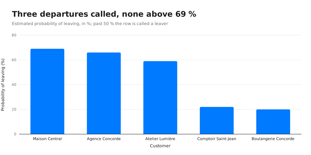
The row-by-row answer, on the customers whose departure status is not consolidated. Three departures called, none above 69 %: each prediction comes with its confidence, and that confidence stays modest.
Before going further, it is worth saying what that 69 % means, because the figure is almost always read wrong. It does not say this customer will leave and that we are 69 % sure of it. It says that among customers resembling this one on the columns observed, about sixty-nine in a hundred left. It is an observed frequency, not a prophecy about a person.
Two quite different things make such a figure uncertain, and confusing them is expensive. The first is our own ignorance: few comparable customers in the history, so an estimate that would move if more data were added. The second is the randomness of the world itself: even granting a perfect history, two customers identical on paper do not make the same decision. The first shrinks by collecting more. The second never shrinks, which is why an honest prediction stays cautious.
From there comes a rule that holds across all three storeys of this chain: a figure without its uncertainty is an opinion dressed as a fact. On this data, no prediction goes above 69 %, and that is a good sign. A tool that had announced 97 % would simply have been lying.
That said, knowing who is leaving without knowing why is useless. You do not keep a customer with a probability, you keep them with a reason. The reason has to be precise enough to act on.
The problem had a name in commerce long before it had one in statistics, and its most famous phrasing fits in a sentence: "Half the money I spend on advertising is wasted; the trouble is I don't know which half." It is credited to the American department-store owner John Wanamaker, sometimes to the British industrialist Lord Leverhulme, occasionally to Henry Ford. The earliest known trace is a 1919 speech already attributing it to Wanamaker, and neither the Wanamaker archives nor Unilever's hold any record of it15. The sentence that states the attribution problem cannot itself be attributed to anyone.
The problem is real enough, and it is ill-posed in the strict sense. The sale happened once. We will never know what would have happened without the poster in the underground, because that world was never observed. Every attribution is therefore a convention: you adopt a rule for splitting, then you live with it.
A small experiment shows how much the choice of rule matters. Two advertising channels, billboards and online, bought together and therefore strongly correlated: 0.84 across two hundred simulated weeks. By construction, only the billboards act on sales; online is a passenger. Then each channel is asked what it explains.

The same channel, the same data, two incompatible answers: the only difference is the order in which the question is asked.
The first two bars say everything. Asked on its own, the online channel explains 55.3 % of the variation in sales, which would make a handsome dashboard. Added to billboards, it explains nothing at all: 0.0 %. That is Wanamaker's trouble, in numbers.
The Shapley split averages over both orders and settles it: 52.5 % to billboards, 27.7 % to online. They sum to 80.1 %, which is exactly what the two channels explain together. That additivity is no happy accident: it is one of the properties Shapley required of his split, and it is what makes the result defensible in a meeting. The protocol is spelled out so you can rerun it instead of taking it on trust: two hundred simulated weeks, seed 20260925, linear regression, the value of a group of channels measured by the share of variation in sales it explains.
One limit remains, and stating it keeps the method from being made to say what it does not. Shapley assigns 27.7 % to a channel we know, by construction, causes nothing. That is not a fault in the method: it answers faithfully the question asked, which is "what did the model use". It does not answer "what caused the sale". For that one there is no shortcut: you need an experiment, cutting a channel's budget in one region and comparing with the others. Attribution explains the model; only experimentation reaches the cause.
The model returned a single number after looking at a dozen columns at once. We would like to be able to say: this much of the 69 % comes from the age of the contract, this much from the number of complaints, this much from the last amount invoiced. Cutting a single result into shares, one per variable that produced it, has a name: attribution. Nothing guarantees in advance that it is possible, because the model did not compute its number as a sum of contributions; it mixed everything together. Attribution reconstructs after the fact a division that never existed in the computation.
The difficulty shows up in the naive attempt. To measure what a variable brings, you can remove it and watch how far the prediction drops. The trouble is that the answer depends on the order in which you remove the others. Removing the age of the contract drops the prediction a long way if nothing has been removed yet, and hardly at all if the number of complaints has already gone, because the two say partly the same thing. So there is not one contribution, but as many answers as there are orders.
Lloyd Shapley solved this in 1953, for an entirely different purpose: sharing a team's payoff fairly among its members, when each brings something different and the contributions overlap16. His answer fits in a sentence: since the order changes the result, consider every possible order and take the average. The picture is a dinner bill. Depending on who arrives first and what gets shared, each person's share changes; averaging over every order of arrival gives a division nobody can dispute. That work earned him the Nobel Memorial Prize in Economic Sciences in 2012. Applied to a prediction rather than a dinner, the same construction says how much each variable weighed, and in which direction17.
The second method starts from a different and equally simple idea. A complicated model stays complicated, but look closely enough, around one single customer, and it behaves almost like a straight line, the way a curve looks straight when you zoom in far enough. So you build, in that small neighbourhood only, a simple model that imitates the big one, then read off its coefficients18, which can be read directly.
Both are shown side by side. When they agree, the reading is solid. When they disagree, that is information in itself: the prediction then rests on a fragile balance between variables, and it is better to know that before calling the customer.
"What is the revenue forecast for the next three months?"
Same foundation, same model, different question. This time the query brings back a series through time; the answer is about months that do not exist yet.
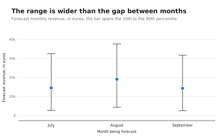
Each forecast month carries its range, from the tenth to the ninetieth percentile. A percentile cuts the possible values into a hundred parts: the tenth is the one below which there is only a one-in-ten chance of landing, the ninetieth the one below which there are nine chances in ten. Between the two, eight chances in ten remain, and that is what the bar says.
A single number about the future is fortune-telling; a number with its range is a decision. And this particular chart says something uncomfortable that has to be read properly: the range is wider than the gap between the three months. August looks better than July, but the bars overlap almost entirely: the gap between the two months means nothing.
That is not a flaw in the tool, it is a verdict on the data. The monthly series in this demonstration database is noise, jumps with no regularity and no pattern behind them: over twenty-one months, 293 euros in one month against 72,380 a year later and three months missing. No method can forecast that; the only honest answer is a wide range. A tool that had returned three neat, tidy numbers would have dressed the situation up. It is the same principle as on the first storey: what is held is not the quality of the answer, it is that its uncertainty is displayed alongside it.
One implementation detail says a lot about the world you work in. The forecast horizon, the number of months to predict, is read out of the user's question, which is to say out of free text. "In a hundred thousand months" translated into a hundred thousand periods to forecast, which means out-of-range dates and a computation that ties up the machine for a result nobody seriously asked for. The horizon is now capped: past that point a forecast has no statistical value anyway, so bounding it removes nothing real.
"Show me where revenue is concentrated"
Last question, last link different: the result is no longer a number or a table, it is a figure. It is chosen automatically from the shape of the data and the intent of the question, then rendered live, with no pre-built dashboard to maintain (those frozen pages of charts prepared in advance). That distinction has a price for whoever decides: a dashboard answers the questions of six months ago, the ones foreseen when it was built.
Except that this choice is exactly where a language model can do anything at all. Show it a hundred and twenty-seven chart names and it can invent one, misspell one or pick one incompatible with the columns present, a map for instance when no column carries geography. The guarantee therefore cannot be a promise of good behaviour. It has to live in the structure itself, where the model cannot miss it.

Two deterministic steps (no model involved, so no surprises possible) bracket the two model calls. The third step eliminates every structurally incompatible candidate before the model sees anything at all; the fourth can only reorder and annotate that already-safe list, never extend it.
The model picks a dish from a menu it did not write. That is a guarantee of a different order from a temperature setting (the dial that makes the model more or less adventurous) or an instruction added at the top of the conversation: it does not depend on the model's compliance, it depends on the shape of the program. And, as on the first storey, it makes the remaining error visible and tractable: a misranked figure is fixed with one click, it does not blend in with a correct one.
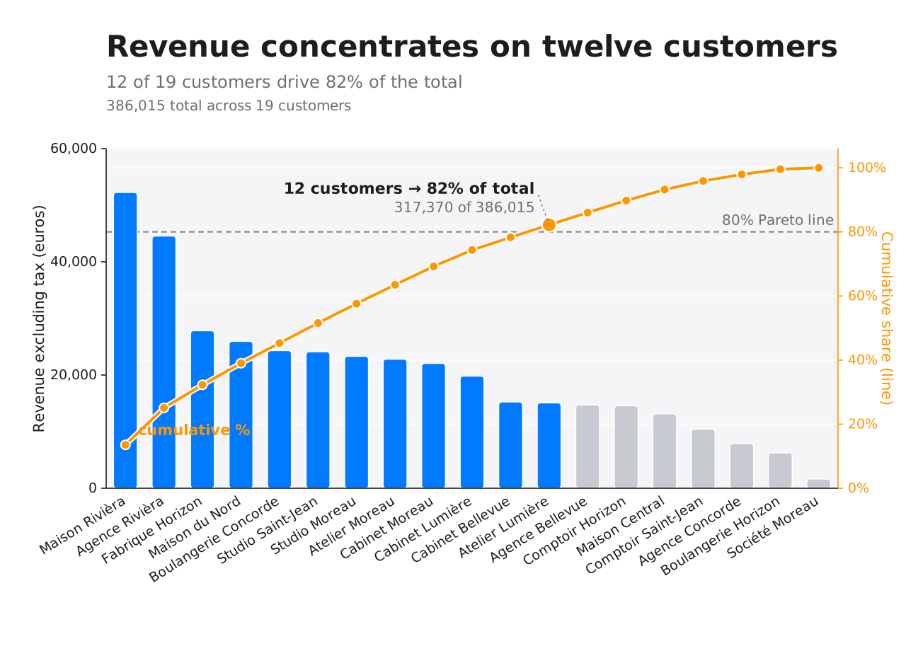
The answer to the question asked: twelve of the nineteen customers the query returned make 82 % of revenue. The cumulative share is over those nineteen customers. That caveat matters: a Pareto chart ranks the contributions from largest to smallest, then draws above them the curve of what they add up to, so you read at a glance how few customers make up most of the total. Drawn on a ranking already truncated upstream, on the other hand, it announces a share "of the total" that is nothing of the kind, for all its neat curve.
The rendering runs on sprezzature.ai, an open source figure engine21. Its catalogue holds a hundred and twenty-seven chart kinds, from lines to sankeys, treemaps, waterfalls, beeswarms and maps. That large number is not hoarding: the wider the catalogue, the richer the list of candidates compatible with the columns present, the more often the automatic pick lands right.
Every figure also meets a standard of accessibility and chromatic rigour: contrast checked, readable under colour blindness, never a colour alone carrying information, the reading direction stated on any axis where up is better than down. None of that is cosmetic. A poorly contrasted chart projected in a room is read by nobody; a chart that requires telling two greens apart excludes one man in twelve. The rules inherited from graphical semiology, the study of what visual forms can convey19, and from perception experiments20, are code here, not recommendations.
What production learns and preparation cannot guess
No amount of upfront curation knows how users will phrase their requests, nor the turns of phrase, shortcuts and special cases proper to each organisation. Production reveals that real distribution of questions. Every question handled well, and above all every correction, is information the initial curation did not have.
The loop is simple to state. A person asks a question, the system produces the query, it runs read-only, a human validates the result or fixes the query. Once validated, the pair joins the library of examples, the index the system draws from. The next similar question then retrieves that new example.
The safety rule is absolute. It is the easiest to get wrong: never blind learning. Automatically capturing every generated query and feeding it back as an example poisons retrieval for every similar question to come. Bad SQL teaches the system to produce bad SQL. A pair is therefore only accepted through a dedicated feedback path, which replays the guardrails and re-executes the query before accepting it: no blind trust, not even in what the caller presents as already verified.
Four properties separate a mechanism that works on one laptop from a production loop. Persistence: the library lives in the database already in place22, not in a memory lost on the first restart. Idempotence: a pair's identifier is computed from its content, so submitting it twice creates no duplicate to clog retrieval. Traceability: every pair that came from the field is marked as such, distinct from the hand-sorted corpus, which makes it possible to audit what production taught the system and to remove one bad example. And measurement: after a batch of additions, you replay the control set. Progress is verified rather than assumed; the control set is what settles it.
What this changes and what it does not
Before, a business question leaves as a ticket for the data team and comes back in three days, often after the decision has been made without it. A predictive question leaves as a project. After, the question is asked out loud, the number lands in seconds, so does the follow-up: the meeting keeps its rhythm. What matters is not that the machine does analysis, it is that the delay between the question and a reliable number drops from three days to three seconds, since the number comes from the database.
What it does not change deserves to be said
just as plainly. The model can still write a bad query. The architecture guarantees read-only access, an allowed syntax tree and bounds; it does not guarantee that the query matches the business intent. On that, it reduces the failure modes and makes them visible, which is not the same as removing them. The real limit is scarcely data volume, since the pipeline goes at the database
rather than an export, with SQL doing the filtering; the limit is the quality of the schema and
the vocabulary. A database whose columns are called col_17 will not let
itself be queried in plain language; no model will change that.
The three lines
txt2sql      question → SQL → database → the real number
txt2sql2ml   question → SQL → table with gaps → the prediction and its range
txt2sql2viz  question → SQL → rows → the right chart, live
One foundation, three storeys. At each one, the same discipline: the model proposes the shape, the machine checks it and the data settles it. That is what separates a number you can sign from a number that merely looks right.
Acknowledgements
Special thanks to Marie Sacksick, Edmond Jacoupeau, Bachir Zerroug and Vincent Sammiez for our fruitful discussions on these topics.
Bibliography
None of these titles is here for decoration: each one carries a design decision taken above. The notes say which.
- Vanna AI. Training advice, project documentation. vanna.ai/docs/training-advice States without hedging the hierarchy of the three materials and the safety rule taken up here: the quality of question-to-query pairs is the single largest determinant of the result and bad SQL learned teaches the system to produce bad SQL.
- Lewis, P. et al. (2020). "Retrieval-Augmented Generation for Knowledge-Intensive NLP Tasks", NeurIPS. arXiv:2005.11401 The paper that named retrieval-augmented generation. It establishes the principle used on the first storey: leave the model untouched and supply, for each question, the context that matters, rather than retraining its weights.
- Vanna AI (2023). How Vanna works, how to train it, data security. medium.com/vanna-ai Walks step by step through the retrieval mechanism everything else depends on: the question is embedded, the nearest knowledge is pulled per content type and only that enters the prompt. This is where the rule "coverage beats volume" comes from.
- Mao, T. sqlglot, SQL parser and transpiler in Python, MIT licence. github.com/tobymao/sqlglot The parser that turns the generated query into a syntax tree before any execution. It is what makes the guardrails possible: you inspect the structure of the query, not a string and refuse anything that is not a read.
- Pourreza, M. and Rafiei, D. (2023). "Evaluating Cross-Domain Text-to-SQL Models and Benchmarks", EMNLP. arXiv:2310.18538 Shows that benchmark scores underestimate models, because a natural-language question admits several correct queries. Justifies the choice of execution match over textual comparison, made here.
- Yu, T. et al. (2018). "Spider: A Large-Scale Human-Labeled Dataset for Complex and Cross-Domain Semantic Parsing and Text-to-SQL Task", EMNLP. arXiv:1809.08887 The benchmark that set the field's habits, starting with evaluation on databases never seen in training. The held-out control set described here is that idea transposed to the scale of a single customer.
- Li, J. et al. (2023). "Can LLM Already Serve as A Database Interface? A BIg Bench for Large-Scale Database Grounded Text-to-SQLs", NeurIPS. arXiv:2305.03111 The BIRD benchmark, built on real databases, dirty and large. It documents the gap between a syntactically correct query and a correct one, which is exactly the gap the column-domain bug exposed here.
- Zavaleta, G. (2026). "Why 90 % accuracy in text-to-SQL is 100 % useless", Towards Data Science. towardsdatascience.com Argues for per-category reading against the global score: a high average accuracy hides the family of queries that fails, which is the family deciding real-world usefulness. It is the reading that singled out joins and one filter here and made the targeted top-up possible.
- NVIDIA. NeMo Agent Toolkit, text-to-SQL, technical documentation. docs.nvidia.com Independently gives the same order of magnitude for the example corpus and the same requirement of validation on a held-out set. Two sources of very different origin converging on "twenty to a hundred well-chosen pairs".
- Brown, T. et al. (2020). "Language Models are Few-Shot Learners", NeurIPS. arXiv:2005.14165 The paper that established in-context learning: one example given inside the conversation is enough to steer the model, without touching its weights. Tabular foundation models transpose exactly that idea from text to tables.
- Hollmann, N., Müller, S., Purucker, L. et al. (2025). "Accurate predictions on small data with a tabular foundation model", Nature, 637, 319-326. 10.1038/s41586-024-08328-6 TabPFN, the German school. Establishes that a model pre-trained once on synthetic tables beats, in a single pass and with no tuning, methods fitted on the data itself. That is the result that makes this second storey possible.
- SAP (2026). SAP Completes Prior Labs Acquisition, press release of 17 July 2026. news.sap.com The acquisition of the Freiburg laboratory, announced in May and closed in July 2026, with more than a billion euros committed over four years. Cited here as a measure of industrial interest in tabular models, not as a technical argument.
- Qu, J., Holzmüller, D., Varoquaux, G. and Le Morvan, M. (2025). "TabICL: A Tabular Foundation Model for In-Context Learning on Large Data", ICML. arXiv:2502.05564 The French school. Column-then-row attention builds a fixed-size representation of each row, which is what lets it hold much larger tables. On a par with TabPFN v2 across two hundred datasets, up to ten times faster and ahead beyond ten thousand rows.
- SODA team, Inria. tabicl, model code and weights. github.com/soda-inria/tabicl The concrete reason for the choice made here: pretraining code, inference code and weights are published, hence auditable and runnable on the customer's own machines, with no data leaving.
- "One-Half the Money I Spend for Advertising Is Wasted, But I Have Never Been Able To Decide Which Half", Quote Investigator, 11 April 2022. quoteinvestigator.com Traces the saying credited to John Wanamaker. The earliest known match is a 1919 speech already attributing it to him; neither the Wanamaker archives nor Unilever's, for the Leverhulme variant, hold any record of it. It is the source for the paragraph on attribution, and the reason this article presents the quotation as apocryphal rather than as a fact.
- Shapley, L. S. (1953). "A Value for n-Person Games", in H. Kuhn and A. Tucker (eds.), Contributions to the Theory of Games II, Princeton University Press, 307-317. The original paper, written to share a team's payoff among its members. It states the axiom that does the work: since the order of arrival changes each share, average over every order. Shapley received the Nobel Memorial Prize in Economic Sciences in 2012, with Alvin Roth. Sixty years separate this text from its use in machine learning.
- Lundberg, S. and Lee, S.-I. (2017). "A Unified Approach to Interpreting Model Predictions", NeurIPS. arXiv:1705.07874 Imports the Shapley value into machine learning, the rule that splits a collective payoff across players by average marginal contribution. Applied to a prediction, it says how much each variable weighed and in which direction.
- Ribeiro, M. T., Singh, S. and Guestrin, C. (2016). "Why Should I Trust You? Explaining the Predictions of Any Classifier", KDD. arXiv:1602.04938 Local surrogate explanation: the model is approximated, in the neighbourhood of the single row under examination, by a simple readable one. Shown here beside the previous method, because two methods disagreeing on one row is a signal in itself.
- Bertin, J. (1967). Sémiologie graphique. Les diagrammes, les réseaux, les cartes, Gauthier-Villars. English edition: Semiology of Graphics, University of Wisconsin Press, 1983. The treatise establishing that a graphical form is not decoration but an encoding and that each visual variable has properties of its own. It is the foundation of the deterministic filter: a figure incompatible with the columns present must never be offered.
- Cleveland, W. S. and McGill, R. (1984). "Graphical Perception: Theory, Experimentation and Application to the Development of Graphical Methods", Journal of the American Statistical Association, 79(387), 531-554. 10.1080/01621459.1984.10478080 Ranks visual encodings experimentally by reading precision, position on a common scale ahead of length, itself ahead of angle and area. It is the measurement that justifies the rules applied automatically to this article's figures.
- Harchaoui, W. sprezzature-figures, open source figure engine. github.com/warith-harchaoui/sprezzature-figures The catalogue of a hundred and twenty-seven chart kinds used on the last storey and the checker that ships with each: contrast, stated polarity, labels that do not collide. The six figures in this article come out of it.
- pgvector, vector search extension for PostgreSQL, PostgreSQL licence. github.com/pgvector/pgvector Lets the knowledge base live in the PostgreSQL already in place, so nothing new has to be deployed. That is what gives the improvement loop its persistence: validated examples survive restarts and are shared across every instance of the service.
- Kong, W., Louidor Ilan, E., Nie, S. et al. (2026). "TabFM: A Zero-Shot Foundation Model for Tabular Data", Google Research, 29 September 2026. arXiv:2609.37959 The third model of the kind, four hundred million internal dials, trained on synthetic tables drawn from causal models. Its result tables carry the TabArena ranking quoted here, where its three variants come ahead of TabPFN-3, AutoGluon and TabICLv2. Measurements run by the authors themselves on a public test bed, to be read as such.
- Google (2026). TabFM Non-Commercial License v1.0, licence of the published weights. huggingface.co The text that settles the question for professional use. It restricts the model to non-commercial purposes, and its definition of the term rules out client deliverables, paid products or services and any revenue-generating activity by name, unless Google grants a commercial licence. Compare with TabICL's BSD licence, which imposes none of these conditions.
- SODA team, Inria. tabicl, licence file. github.com/soda-inria/tabicl Three-clause BSD for the most part, with one declared exception: the forecasting directory is a derived work from TabPFN-TS and stays under an Apache licence in Prior Labs' name. Concrete proof that the two schools read each other, in a document nobody writes for show.
Two books to widen the view. My favourite AI books, for the guided overview. Edward Tufte's The Visual Display of Quantitative Information, for everything the last storey automates without being able to replace it: the judgement about which question the figure should ask.