In short
Reinforcement learning (RL) teaches a machine to act by trial and error, guided by a numerical reward. In 2018, Joelle Pineau showed two major conferences why the published results of this field inspired little trust. We took up her list of sixteen flaws with two instruments. The first rereads the papers from 2018 to 2026 with her reading grid, the list of criteria she scored in each paper. The second reruns her experiments under a protocol, an experimental plan written in advance. Our answer, after reading eight years of papers, rerunning her experiments and proposing new ones: Pineau was heard on what gets published alongside the result, much less on how to judge the result itself.
- What changed. In classical RL, the RL of robots and simulated games, with the same reading grid on both sides, linking the code went from 31% to 74% of papers, quantifying the compute (how much computation the experiments needed) from 27% to 58%, showing the effect of a setting (how the result moves when a setting changes) from 44% to 80%, reporting an uncertainty from 63% to 88%. This last rise is the most fragile: it does not withstand all our checks, the analysis redone with one choice changed.
- What shows no detectable change. The statistical test (6% then 12%), baselines (the methods a paper compares itself with) described with all their settings, evaluation on held-out conditions the agent never saw during training.
- The contribution of our experiments. When the same program is launched several times, each complete training is a run. Two groups of these runs drawn at random rarely fool a statistical test. Two sorted groups, the best on one side and the worst on the other, fool it nearly one time in three. Keeping the best three runs out of ten inflates the mean by a third. The t of 9 from 2018, the statistical test result that passed off two groups of the same program as two algorithms, most probably comes from a test that counts the games the program plays during its training (the episodes) instead of the independent training runs (the random seeds).
Two curves, one program
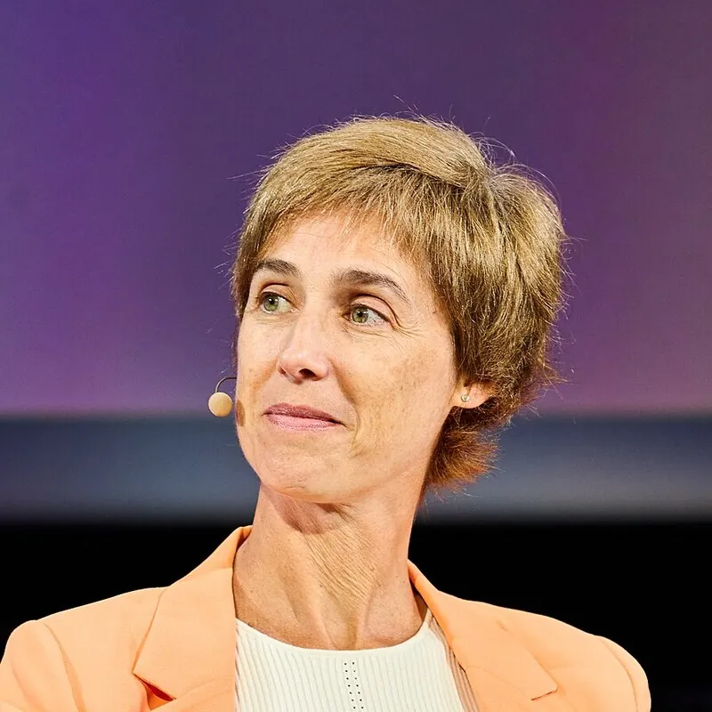
In the spring of 2018, in Vancouver, Joelle Pineau walks onto the stage of ICLR, one of the three major conferences of machine learning1. She is a professor at McGill University and runs Facebook's artificial intelligence research lab in Montreal. In December, in Montreal, she takes up and extends her talk before NeurIPS, the largest of the three2.
The Vancouver talk, in full.
She shows two learning curves. An articulated cheetah, drawn in two dimensions inside a physics simulator, learns to run. Each curve follows the cheetah's score over training, averaged over five runs. The two curves pull clearly apart. A statistical test, the calculation that judges whether a gap could come from chance, declares them different: t = −9.09, p = 0.0016. These two numbers, explained in the next section, say that chance would be a very poor explanation for such a gap. A reviewer of scientific papers would see two algorithms, one better than the other.
Yet both curves come from a single program, the learning algorithm TRPO, with the same settings. Only the random seed changes, the starting number from which the computer draws all the chance in a training run. Pineau says on stage that the two groups of five runs are not sorted: they are "just five runs" on each side. Chance alone produced a publishable "improvement".
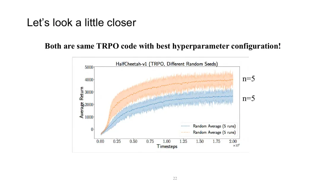
Two groups of five training runs of the same TRPO program on HalfCheetah, differing only in their random seed.
Joelle Pineau, NeurIPS 2018, page 22 of her slides, after Henderson and coauthors (2018).
The two-curve figure is taken from a paper by her team, signed by Peter Henderson and his coauthors3. It serves a broader point. Pineau starts from a survey by the journal Nature: of 1,576 researchers from every discipline, more than 70% said they had already failed to reproduce a colleague's experiment4. She then quotes two Stanford researchers, Buckheit and Donoho, who wrote in 1995 that a scientific paper about computation is merely the advertising of the research. The research itself is the complete software and the instructions that produced the figures5. Then she shows, figure after figure, what her field lacks to deserve trust.
The cheetah, the random seed and the test
A program, the agent, acts in a simulated world. At each step, it observes a situation, chooses an action and receives a numerical reward. It looks for the way of acting that pays the most in total. The cheetah of the slide is called HalfCheetah: the agent drives its six joints and scores points when the cheetah moves forward. At first it wriggles, after a million steps it runs. Three other simulated bodies appear in our experiments. Hopper hops on one leg, Walker2d walks on two legs and Swimmer swims.
Training draws many numbers at random, from the starting parameters of the neural network, the numbers that learning adjusts bit by bit, to the actions tried out to explore and the initial position of the cheetah.
Same program, same random seed: same result.
Same program, another random seed: another result.
A "run" here means a complete training with a given random seed.
The settings the experimenter fixes by hand, such as the learning rate or the size of the network, are called hyperparameters. To show that a new method does better, a paper compares it with existing methods, the baselines. The comparison is fair when all of them received the same care in tuning.
The mean scores of two methods always differ a little, even when the two methods are identical. A statistical test says whether the observed gap exceeds what chance usually produces. To do so it computes a number, the t: the gap between the two means, divided by the variation chance usually produces. The larger the t, ignoring its sign, the sturdier the gap looks. From the t, the test derives the p-value, the probability of seeing a gap at least this large if the two methods were in truth equivalent. Below 0.05, one chance in twenty, researchers call the gap "significant" by convention. With two groups of five runs, a t of three already clears that threshold. A t of 9 is therefore enormous. It is the one on the 2018 slide, sign aside. A 95% interval gives the range where the true size of the gap very probably lies. If it contains zero, the gap may be nothing but chance.
Sixteen flaws in four families
Pineau shows each flaw with an example. We found sixteen in her two talks, sorted into four families.
- The material. The paper comes out without its code, without the exact settings or the compute required, without the versions of the software used, on which the result also depends.
- The tuning. Hyperparameters are given in part, how they were chosen goes unsaid. Baselines get less care than the method being defended.
- Random seeds and statistics. Papers launch three or five runs, never ten in the table she shows. Only the best runs are published. Two groups of the same code look like two algorithms. No statistical test is applied.
- The reach of the conclusions. The best algorithm changes from one task to the next. Two programs coding the same algorithm give different results. The agent is evaluated in the very world it trained in, on benchmarks (the standard tasks everyone compares on) so simple it learns them by heart.
Eight years have passed. In 2019, NeurIPS adopted the checklist Pineau proposed, a set of questions every author fills in when submitting a paper6. Did we listen to her? Two instruments answer. One rereads papers with her reading grid, extended by a second grid for the flaws her grid did not measure. The other reruns her experiments with the algorithms of 2026, under a protocol written before the first training run: every later change is logged there with its date and reason.
Most of our experiments use ten random seeds, hence ten runs, per program and per task. We then reran them with twenty. The protocol had fixed in advance that the first ten are authoritative: the numbers below come from those ten random seeds. We flag every place where the twenty qualify a result.
Reread 2018 before judging 2026
Pineau had read 50 RL papers from 2018 and scored eight criteria for each. We took every paper of the three major conferences, ICLR 2026, ICML 2026 and NeurIPS 2025, whose title mentions reinforcement learning, or 1,252 out of 17,836. A first random draw kept 50. Among them, 27 apply what they call RL to large language models, 14 belong to classical RL (robotics, games, machine control) and 9 are theoretical. Large language models are the generative AI models that write text, like ChatGPT. We drew more classical RL papers, up to 50, because fourteen are too few to detect a gap of thirty points.
Who read these papers? Generative AI programs, of the same family as ChatGPT. We salute these new readers, who even read the appendices. For each paper and each criterion, the reader decides yes or no, with an exact quotation from the paper and its page, which anyone can check in the project's online repository. Ten papers were reread by a second reader blind to the first reading. The two readers agree on 127 decisions out of 130 (98%). Since all these readers are copies of the same generative AI model, this agreement measures the model's consistency. No human redid the reading independently. A "no" could also hide a reader's oversight. With keywords fixed in advance, we searched for whatever could contradict each "no". Of 377 "no" decisions, 10 turn into "yes", 2 in 2018 and 8 in 2026. No verdict changes: our conclusions about the practices stay the same.
One gap separates us from Pineau herself. We reread 50 papers from 2018 with her reading grid. Our reading finds 55% of papers giving all the settings of their method, where Pineau counted 90%. Comparing our 2026 papers with her numbers would mix two changes, that of practice and that of the reading. Each verdict therefore compares classical RL in 2026 with the 2018 papers as we read them, with the same grids and the same readers.

Gap, in percentage points, between 50 classical RL papers from 2026 and 50 papers from 2018, read with the same grids by the same readers. The dot gives the observed gap, the bar its 95% confidence interval.
The four practices in green have intervals that avoid zero.
Four practices changed. Linking the code went from 31% to 74% of papers, showing the effect of a setting from 44% to 80%, quantifying the compute from 27% to 58%, reporting an uncertainty (error bars or a band around the curve) from 63% to 88%. Comparing eight practices gives chance eight opportunities to produce a false gap. We therefore tightened the threshold below which a gap counts, as is customary in that case. We also redid the analysis several ways, changing one choice each time. These variants are our checks. Code and compute clear the threshold in every check, the effect of a setting in almost all. The rise in uncertainty is fragile: two of our checks make it fail, with p = 0.07 each time, above the threshold.
The other practices show no detectable change. The statistical test goes from 6% to 12%, baselines described with all their settings from 35% to 29%, evaluation on held-out conditions from 33% to 45%, the benchmark version from 23% to 26%. With 50 papers on each side, a change of ten points can still go unnoticed: "no detectable change" does not mean "no change". One contrast, however, is sharp. Nearly every paper now draws error bars, very few apply a statistical test.
A slow climb that began before the checklist
Comparing two years does not say when, in between, the change happened. So we read 20 classical RL papers per year from ICML and NeurIPS, in 2019, 2020, 2022 and 2024, drawn at random and read with both grids.

Share of classical RL papers following each practice, year by year: 48 papers from 2018 (those with experiments), 20 per year from 2019 to 2024, 50 from 2026. With 20 papers, a share is uncertain by about twenty points either way.
The four upper practices climb steadily. The statistical test, in grey, shows no trend.
The four practices climb with no clear jump right after the 2019 checklist. The effect of a setting is an exception: it rises later, from 40% over 2019 and 2020 to 73% over 2022 and 2024. These series describe a slow rise that began before the checklist or with it. They do not say what caused it.
The checklist had a surprise in store for us. Every NeurIPS paper attaches the checklist filled in by its authors. Of the 30 NeurIPS 2025 papers we had read, we compared these answers with the text of the paper. The checklist's question on statistical significance (testing) settles for error bars "or other appropriate information". The 18 papers that answer yes to it apply no test. On code, 5 papers out of 22 answer yes without a link to their code. A ticked box does not guarantee the practice it names.
Another surprise: what moved is not always the easiest. Showing the effect of a setting takes extra training runs. The practice progressed despite that cost. Giving a benchmark's version takes one line of text, which is missing as often as before.
Thirty random seeds, one program
Rereading the papers told us what changed in publications. Our experiments now put the flaws to the test, starting with the most famous, the two curves from one program. We redid the 2018 experiment on a larger scale: thirty training runs of PPO, one of the most widely used reinforcement learning algorithms, on HalfCheetah, a million steps each, with the same code and the same hyperparameters. Between two training runs, the random seed differs and nothing else.

Thirty training runs of the same program on the same task, PPO on HalfCheetah. Each dot is a run, placed at its final score. Only the random seed changes from one dot to the next.
Mean 1,688, median 1,580.
The mean is 1,688. The standard deviation, which says how far a run usually strays from the mean, is 568, or 34% of the mean. Twenty-seven runs end between 1,138 and 1,999, three take off beyond 3,000. Not one line of the program changes from one run to the next. Yet the scores do not draw a bell curve, the shape where they would bunch symmetrically around the mean: the runs that take off pull the mean above the median, the score of the middle run.
We then drew two groups of equal size from these thirty runs 10,000 times, then applied Welch's test to each pair of groups, the most common test for comparing two means. Both groups come from the same program: every gap declared significant is an error of the test, a false positive.

Share of the 10,000 draws where the test declares two groups of runs of the same program different, at the usual 5% threshold.
Drawn at random, the groups fool the test less often than this threshold. Sorted, they fool it nearly one time in three.
The result defies what the slide led us to expect. Two groups of five drawn at random almost never fool the test, in 1.2% of the draws. They fool the eye, though. Their means differ by 17% at the median and by 47% one time in twenty, enough to draw two well-separated curves. The test gives way when we sort: setting the five best runs against the five worst gives 31% false positives. Chance fools the eye, sorting fools the test.
The riddle of the t of 9
Where, then, does the t of 9 from 2018 come from, if groups drawn at random so rarely fool the test? Henderson and his coauthors did not test final scores. Their caption speaks of an average t over the whole learning curve: the test is rerun at each point of the curve, then the t values are averaged. We redid this computation on our thirty curves. One time in twenty, this average t exceeds 1.4 when the groups are drawn at random, 2.5 when they are sorted. None of our 20,000 draws reaches 9.
First lead: with their algorithm, TRPO, scores may vary more from one random seed to the next than with PPO. We trained TRPO thirty times, with a plan written before any training. Its scores vary far more, since its standard deviation is 48% of its mean. Despite that spread, the average t exceeds 1.4 only one time in twenty at random, 1.9 sorted. The second lead is another way of computing t, which stacks the points of each group's five curves, a hundred in all, as if every point came from a separate run. Its t, one time in twenty, climbs to 5.0 at random and 6.3 sorted. Worse, this computation declares a difference in 53% of the random draws, between two groups of the same code. None of these computations reaches 9.
The published number held the clue. A t of 9.09 with p = 0.0016 implies about 3.4 degrees of freedom, a setting of the test that depends on how many measurements are compared. Yet comparing two groups of five runs always gives at least 4 degrees of freedom. At 3.4, this number cannot come from comparing five runs with five runs. It gives away a different computation. In June 2017, Peter Henderson had published a small program, a script, with a telling name: "from the same distribution"7. The script averages the curves of the five random seeds of each group. Then, at each point of the curve, it compares the two groups with a test built on how much scores vary between episodes, the successive games one agent plays during training. The variation between random seeds, the one the figure was meant to show, never enters the test.
The eureka moment
We applied this script to our thirty TRPO runs, with a plan written before the computation. The average t exceeds 9.09 in 38% of random draws. The test declares a difference in 43% of the cases. The 2018 number comes back out of our own runs.
Recall that the t divides the gap between two groups by the variation the test measures. Measuring the variation between episodes is like comparing the average height of two classes while trusting the precision of the tape measure instead of the height differences between pupils. The smallest gap between the two classes then looks immense. The episodes of one agent play the part of the tape measure, the random seeds that of the pupils. In our TRPO, the standard deviation between episodes of the same agent is 7% of the standard deviation between agents, or between random seeds: divided by so small a variation, the same gap yields a huge t. With PPO, whose episodes vary more, the same computation never reaches 9.

Two groups of five runs drawn at random from thirty, 10,000 times, for each algorithm and each way of computing t. The bar gives the share of draws where the average t, sign set aside, reaches 9.09, the number published in 2018.
Only the 2017 script, applied to TRPO, gets there.
Nothing proves this script produced the 2018 figure. Its name and the numbers it outputs make it likely. The t of 9 needed no sorting: a test that counts episodes instead of random seeds is enough to produce it. The flaw runs deeper than the figure said. The chance of the random seeds fooled the very test meant to measure it.
Keep the best, inflate by a third
Pineau showed another practice. Authors do ten training runs and publish the mean of the best ones. Every published score was really obtained. Their mean still exceeds what the method usually gives. From our thirty PPO runs, we drew ten runs at random, a great many times. Averaged over these draws, keeping the best three out of ten inflates the mean by 33%: 2,249 instead of 1,692.
The same selection is then applied to four programs on four tasks, ten random seeds each. They are two versions of PPO, written with two different computing toolkits (PyTorch and JAX), then SAC and CrossQ, a descendant of SAC published in 2024. The tasks are HalfCheetah, Hopper, Walker2d and Swimmer.

Rise of the mean when only the best three of ten runs are published, for each program and each task.
All sixteen rises are positive: sorting always serves whoever does it.
The mean inflates by 32% at the median, from 6% to 84% depending on the program and the task. Of 24 comparisons between two programs, 3 flip: the loser becomes the winner. Two of them pit the two versions of PPO against each other. When the gap is small, keeping one's best runs is enough to change the winner. Redone on ten other random seeds, the same selection inflates the mean by 43% at the median and again reverses 3 comparisons out of 24.
In papers, the practice rarely shows: 14% of classical RL papers from 2026 let it show, against 19% in 2018. These shares are lower bounds, since a paper that keeps its best runs without saying so escapes our reading.
How many runs do papers launch? Of 41 experimental RL papers in the first 2026 draw, 20 do not say how many, 4 have only one and the median of the others is five, the most frequent value in Pineau's table. The number has not moved in eight years. Yet between two of our programs whose means differ by less than 20%, five random seeds recover the right order only 71 times in a hundred at the median. Measured on our twenty random seeds, this figure falls to 62 times out of a hundred. Such a gap reads backwards more than one time in three.
The leading program depends on the task and on the budget
In 2018, Henderson and his coauthors showed that the leading algorithm on HalfCheetah stopped leading on Hopper or Swimmer. With our four programs of 2026, the leading program also changes from one task to the next. Each score is an interquartile mean: drop the lowest quarter and the highest quarter of the ten runs, then average the rest, so that no single outlying run drags the score by itself8.

Score of each program relative to the best on its task, over ten random seeds: the bar at 100 marks the leader.
PPO trains for a million steps, SAC and CrossQ for 200,000.
SAC leads on HalfCheetah, PPO written in JAX on Hopper and Swimmer, CrossQ on Walker2d. The same SAC is far behind on Hopper and on Walker2d. Yet the leading program clearly beats all the others only on Walker2d: on the three other tasks, ten random seeds are not enough to separate it from the runner-up.
One detail of the protocol weighs heavily: the budget, the number of training steps. PPO trains for a million steps, five times more than SAC and CrossQ. To compare at equal budget, we also read PPO's score at 200,000 steps, under a rule written before looking at these scores. PPO then leads on no task. With ten random seeds, SAC still holds the lead on HalfCheetah. With twenty, CrossQ comes first on all four tasks, without its lead over SAC on HalfCheetah being settled. The ranking depends on the task, but also on the budget each program receives. A paper that compares two methods at different budgets compares those budgets too.
The two versions of PPO, the same algorithm programmed with two toolkits, do not get the same score either. On Walker2d, PPO written in PyTorch scores 2,158, PPO written in JAX 1,272, or 41% less. The two intervals still overlap with ten random seeds: ten do not tell which version does better. A method whose score fell between the two would win or lose against "PPO" depending on the version chosen. With twenty random seeds, the decision rule fixed in advance names a winner on two tasks. PPO written in PyTorch wins on Walker2d, with 2,204 against 1,435. PPO written in JAX wins on Swimmer. The same algorithm, two toolkits, two winners.
Twenty percent heavier
The ranking shifts with the task, with the budget and with the version of the program. Pineau also asked that training be kept apart from evaluation. A student who saw the exam the night before can pass without understanding anything. In RL, the agent is often evaluated in the world it trained in. It is that student, who may have learned this world by heart. We evaluated our agents twice, with random seeds never seen in training: in the physics of their training, then with masses 20% heavier and friction 20% lower.

Hopper, four programs, ten random seeds each. On the left, the score in the training physics. On the right, the score with heavier masses and lower friction.
Ranks compare interquartile means, without a test.
Twelve program-task pairs out of sixteen lose a detectable share of their score, that is, a drop the chance of the random seeds does not explain. The loss depends on the program. On Hopper, PPO keeps only 22% of its score in its PyTorch version and 18% in its JAX version, while SAC keeps 64% and CrossQ 65%. These shares are computed run by run, then summarized with the same interquartile mean, which does not give exactly the ratio of the two scores in the figure. PPO written in JAX, first on Hopper in the training physics, ends last in the modified physics. CrossQ takes the lead there.
To check this reversal, we wrote a rule before any new computation: re-evaluate each agent changing one quantity at a time, masses from 30% lighter to 30% heavier, friction from 40% lower to 20% higher. A pair loses when it does worse than in the training physics beyond what the chance of the random seeds explains. In precise terms, the 95% interval of its score relative to the training physics stays below 1.

Four programs on four tasks, ten random seeds each, or 16 pairs of program and task. Each point counts the pairs that lose a detectable share of their score when a single quantity of the physics changes, masses or friction.
A pair loses when the 95% interval of its score relative to the training physics stays below 1. At 0%, the training physics serves as the reference: no loss is possible there.
The loss grows as the physics departs from training and draws a V. Masses 10% lighter cost 3 pairs out of 16 a detectable share of their score. Made 20% heavier, they make 12 lose. Friction matters less, except 20% higher: 9 pairs lose there. On Hopper, PPO written in JAX is no longer first in 10 modified physics out of 12, with ten random seeds as with twenty. The reversal holds.
Have papers changed on this point? In classical RL, evaluation on held-out conditions goes from 33% to 45% of papers, a rise too small to tell apart from sampling chance. Held-out evaluation has become the rule elsewhere, in the papers that apply these methods to large language models, whose problem sets separate training and test from the start.
A baseline a little too good to be true
Pineau's criteria apply to ourselves first. One of our experiments was meant to illustrate a poorly tuned baseline. It sets two PPOs against each other on Hopper. The first keeps the default values of its software library, the ready-made software we take PPO from. The default values are the settings this library uses when nothing is tuned. The second takes the settings published by the RL Baselines3 Zoo collection, the reference for this library9. First result: 2,877 for the default values, 1,003 for the tuned version. The published settings would do nearly three times worse than the defaults?
The result was too good to believe without checking. We found an error on our side. Our code prepared the data the agent sees with a setting of 0.99, where the collection uses 0.999. Our error was real, but it explained nothing. With the error fixed, the published settings do just as badly. Ten agents trained with the collection's official script score 995, against 2,423 for the default values, both groups trained this time on the benchmark version the collection was tuned for. Our most likely explanation: the published recipe has aged, because the software around it has changed since it came out. A result that looks too good gets checked to the end.
A coin-flip reward
Until now, all our experiments took place on simulated bodies, the kind on which robotics often works out its movements before handing them to real robots. RL's vocabulary has also reached the generative AI models that write text, like ChatGPT: some of RL's algorithms are borrowed (with a vague resemblance) to fine-tune their answers, with no agent acting in a world. They are given a math problem, a program checks the answer, the right ones are rewarded. In 2025, a team at the University of Washington showed that a reward drawn at random, without looking at whether the answer is right, improves Qwen models in mathematics, but not Llama or OLMo models10. On Qwen2.5-Math-7B and the MATH-500 benchmark, the true reward, the one that pays for right answers, gains 29.1 percentage points, a reward drawn at random 21.4. A coin that learns mathematics?
We wanted to see the phenomenon up close, at small scale. We wrote GRPO ourselves, one of the most widespread training algorithms for this use11 and applied it to two small open models that anyone can download: Qwen2.5 with 0.5 billion parameters and Llama 3.2 with 1 billion. Each model trains for a hundred steps, each step nudging its parameters a little, with the true reward, then with a coin-flip reward. We launched three random seeds each time, before adding two more.

Share of problems solved at the first attempt, at the start and after a hundred training steps, for each model, each reward and each of the five random seeds.
With the true reward, the same program gives very different results from one random seed to the next. With a coin flip, success falls to zero or nearly.
With a coin flip, the answer is plain: success falls to 1% or less in all nine finished runs. The tenth, a Llama run, stopped twice at its first step, on a safeguard that halts training when its computations run away. We count it among the results, on the same footing as the other nine. Here, heads or tails, the coin always lands on the wrong side.
With the true reward, the story comes in two acts. Over three random seeds, Qwen starts at about 10% and ends at 36%, 61% and 13%: the 2018 random-seed flaw in miniature, one program giving three very different results. The mean gain is +26 points, with an interval from +2 to +51.
With two more random seeds, the new runs end at 13% and 0%. Over five random seeds, the mean gain drops to +14 points, with an interval from −3 to +34: it contains zero. Two runs were enough to undo the result.
The early gain rested on the first two runs, done on the GPU. The three runs that ran on the CPU, after GPU crashes, have a mean gain of −2 points. Hardware and random seed are tangled together there: with five runs, we cannot tell whether the gap comes from the machine or from the luck of the random seed. On Llama, the mean gain is +6 points, from just below zero to +15. This part of our experiments remains an illustration on small models, far from a replication of the Washington team.
The cutoff trap
Our GRPO training brought a benchmark trap to light. The model's answers are cut at 160 tokens, the word pieces it produces one by one. With the base model, before any training, 23 answers out of 32 hit this limit before giving a result. None of these cut answers is right.

The answers of the Qwen2.5 model with 0.5 billion parameters before any training, eight per problem.
Most hit the 160-token limit before giving a result and count as wrong.
With the true reward, the model learns to finish before the cutoff: over the ten runs, the share of cut answers ends between 0% and 29%. With a coin flip, it ends above half in six runs out of nine, between 2% and 16% in the other three. But a cut answer counts as wrong. A model that learns to answer more briefly gains points without calculating any better. Part of the measured "gain" may therefore come from a detail of the benchmark, learning to stop talking in time. We now measure the share of cut answers at every evaluation.
Listened to in part
Joelle Pineau was heard on what gets published alongside the result: the code, the compute, the effect of a setting. She was heard much less on how to judge the result itself. The test remains rare, baseline settings remain poorly described, evaluation still often happens in the training world.
Our experiments sharpen the most famous flaw. Random seeds produce visible gaps. Two choices by the experimenter make them worse: sorting the runs turns these gaps into false positives, keeping the best inflates the mean. The t of 9 has, in all likelihood, another origin, a test that counts episodes instead of random seeds. We draw three rules from this:
- never sort random seeds before comparing;
- show an interval next to every curve;
- apply the test to the gaps between random seeds, never to the gaps between episodes.
Two traps lay in wait for us in turn: a result too good to be true, where we found an error in our own code that explained nothing, then a first indicator on language models that also measured a length limit. The protocol written in advance put us on the trail of the code error, while checking surprising results led us to the length limit. And the protocol keeps a dated record of every correction. Anyone can see what we changed and why. In 2018, Pineau advised being as critical of your good results as of your bad ones.
Seven questions for reading an RL claim
The checklist is meant for authors. Anyone reading a paper, a press release or a demo can draw seven questions from it, which require no programming.
- How many random seeds? With fewer than five runs, or with "the best runs", the result says little.
- What uncertainty? A mean with no interval and no band around the curve does not allow a gap to be judged.
- Which baseline, tuned how? If the method got a month of tuning and the baseline its default values, the gap measures the month of tuning.
- What budget? Comparing two methods trained on different numbers of steps also compares those numbers of steps.
- Evaluated where? An agent judged on the situations of its training may have learned them by heart.
- What code? Without published code, nobody knows what the paper really did.
- What compute? A result that nobody else can afford to recompute cannot be reproduced.
The full document and the code
This article summarizes a much longer document, which goes through the sixteen flaws one by one, with all the numbers, their intervals and their limits: the full document (PDF). The code, the protocols written in advance, the training logs, the paper readings with their quotations and the scripts that regenerate every figure are in the project repository12.
Our verdicts hold for classical RL, read by generative AI programs on fifty papers on each side. A change of ten points can still go unnoticed there. Joelle Pineau asked that criticism apply to oneself first: our work is online, number by number, for anyone who wants to redo it.
Let's talk AI.
The figures in this article were made with sprezzature.ai by Deraison.ai
 sprezzature.ai
 Deraison.ai
Bibliography
Each title below served one specific section. Its note says which.
- Pineau, J. (2018). Reproducibility, Reusability, and Robustness in Deep Reinforcement Learning. Invited talk, ICLR 2018, Vancouver. iclr.cc The Vancouver talk, where Pineau presents the flaws of deep RL.
- Pineau, J. (2018). Reproducible, Reusable, and Robust Reinforcement Learning. Posner Lecture, NeurIPS 2018, Montreal. Slides The Montreal version: the slide of the two groups of five runs, the grid of the fifty 2018 papers and the checklist.
- Henderson, P., Islam, R., Bachman, P., Pineau, J., Precup, D. and Meger, D. (2018). Deep Reinforcement Learning that Matters. AAAI 2018. arxiv.org The written source of the figures: the two groups of five random seeds, the ranking by task, the implementations that diverge.
- Baker, M. (2016). 1,500 scientists lift the lid on reproducibility. Nature, 533, pp. 452-454. nature.com The survey of 1,576 researchers on reproducibility that opens the talk.
- Buckheit, J. B. and Donoho, D. L. (1995). WaveLab and Reproducible Research. In Wavelets and Statistics, Springer, pp. 55-81. doi.org The sentence about the paper as mere advertising of the research.
- Pineau, J., Vincent-Lamarre, P., Sinha, K. et al. (2021). Improving Reproducibility in Machine Learning Research (A Report from the NeurIPS 2019 Reproducibility Program). Journal of Machine Learning Research, 22(164), pp. 1-20. jmlr.org The adoption of the checklist by NeurIPS in 2019.
- Henderson, P. (2017). from_same_dist.py, repository ReproducibilityInContinuousPolicyGradientMethods. GitHub. github.com The script that tests the spread between episodes and finds the t of 9.
- Agarwal, R., Schwarzer, M., Castro, P. S., Courville, A. and Bellemare, M. G. (2021). Deep Reinforcement Learning at the Edge of the Statistical Precipice. NeurIPS 2021. arxiv.org The interquartile mean and the resampling intervals used in our experiments.
- Raffin, A. (2020). RL Baselines3 Zoo. github.com The collection of published settings whose recipe has aged with the libraries.
- Shao, R., Li, S. S., Xin, R. et al. (2025). Spurious Rewards: Rethinking Training Signals in RLVR. arxiv.org The reward drawn by chance that improves Qwen, but neither Llama nor OLMo.
- Shao, Z., Wang, P., Zhu, Q. et al. (2024). DeepSeekMath: Pushing the Limits of Mathematical Reasoning in Open Language Models. arxiv.org The GRPO algorithm, which we wrote ourselves for the language model part.
- Harchaoui, W. (2026). Reinforcement Learning: Did We Listen to Joelle Pineau in 2018? Full document, protocols, data and code. Project repository The document this article is drawn from, with every number and its sources.